Chapter 2. Angular Momentum.

or, as in Eq. (2.32), a spin-down electron can be labeled with a horizontal bar, $χ_{2} (x) = \overline{ψ} (r)$ , and the absence of a horizontal bar identifies a spin-up electron, $χ_{1} (x) = ψ (r)$ . The spatial part of the spin-orbital, $ψ (r)$ , is referred to as an atomic orbital (AO) for many-electron atoms and as a molecular orbital (MO) when applied to molecules.

The total wavefunction of a one-particle system can be written as a two-component spinor

(2.41)

Ψ (r) = (\begin{matrix} 〈 r, σ = ↑ | Ψ 〉 \\ 〈 r, σ = ↓ | Ψ 〉 \end{matrix}) = (\begin{matrix} Ψ_{↑} (r) \\ Ψ_{↓} (r) \end{matrix}),

which can also be expressed in terms of the spin eigenvectors as

(2.42)

Ψ (r) = Ψ_{↑} (r) (\begin{matrix} 1 \\ 0 \end{matrix}) + Ψ_{↓} (r) (\begin{matrix} 0 \\ 1 \end{matrix}) = Ψ_{↑} (r) α + Ψ_{↓} (r) β .

$Ψ_{↑} (r)$ and $Ψ_{↓} (r)$ are the spatially dependent amplitudes of the single-particle being in the spin-up state and spin-down state, respectively; ${| Ψ_{↑} (r) |}^{2}$ is the probability of a particle being located at position r with it's spin up, and ${| Ψ_{↓} (r) |}^{2}$ is the probability of it being at a position r with its spin down. For any system of identical fermions, such as many-electron atoms and molecules, the Pauli principle requires that the wavefunction must be antisymmetric. In the next section, the N-electron wavefunctions will be approximated by Slater determinants, which uphold, by design, the antisymmetry requirement. In a N-electron system, each spin-orbital can be occupied by any one of the electrons. The total wavefunction of the N-particle system will be constructed with N spin-orbitals of the form described above.

[Back to Table of Contents] [Top of Chapter 2] [scienceelearning.org]

2.3. The total angular momentum.

The total angular momentum, excluding nuclear spins, is represented by the symbol $\hat{J}$ . For atoms, $\hat{J} = \hat{L} + \hat{S}$ , where $\hat{L}$ is the orbital angular momentum operator. This can also be written as

(2.43)

\hat{J} = \hat{L} \otimes 1 + 1 \otimes \hat{S}

to emphasize that $\hat{L}$ and $\hat{S}$ operate on different spaces. $\hat{L} \otimes 1$ is the direct product of the orbital-angular momentum operator ( $\hat{L}$ ) of a Hilbert space spanned by position kets and the identity operator (1) of a two-dimensional spin vector space. Similarly, $1 \otimes \hat{S}$ is the direct product of the identity operator (1) of a Hilbert space spanned by position kets and the spin angular momentum operator ( $\hat{S}$ ) of a two-dimensional spin vector space. One immediate consequence of the fact that $\hat{L}$ and $\hat{S}$ operate on different spaces is that the two operators commute, i.e., $[\hat{L}, \hat{S}] = 0$ . Equation (2.43) is really the total electronic angular momentum. For our purposes, individual nuclei can be treated as spherically symmetric point particles, but for molecules the rotational angular momentum of the nuclear framework must also be considered. In this case, the total angular momentum operator, excluding nuclear spin, is given by $\hat{J} = \hat{R} + \hat{L} + \hat{S}, where \hat{R}$ is the nuclear rotational angular momentum operator [see Appendix A]. For molecules, ${\hat{J}}_{a} = \hat{L} + \hat{S}$ is only the total electronic angular momentum, and, of course, for atoms $\hat{J} = {\hat{J}}_{a}$ .

All the operator relationships described previously for spin angular momentum can be generalized to the total angular momentum. $\hat{J}$ can be written in terms of its Cartesian components as

(2.44)

\hat{J} = {\hat{J}}_{x} \hat{x} + {\hat{J}}_{y} \hat{y} + {\hat{J}}_{z} \hat{z},

from which we can define the operator ${\hat{J}}^{2}$ as

(2.45)

{\hat{J}}^{2} = {\hat{J}}_{x}^{2} + {\hat{J}}_{y}^{2} + {\hat{J}}_{z}^{2} .

It will also prove useful to define the following ladder operators

(2.46)

{\hat{J}}_{\pm} = {\hat{J}}_{x} \pm i {\hat{J}}_{y} = {\hat{J}}_{\mp}^{†},

which are particularly useful for establishing the properties of the of angular momentum operators and their eigenstates. ${\hat{J}}_{x}$ and ${\hat{J}}_{y}$ can be written in terms of the ladder operators as follows

(2.47)

{\hat{J}}_{x} = \frac{{\hat{J}}_{+} + {\hat{J}}_{-}}{2} and {\hat{J}}_{y} = \frac{{\hat{J}}_{+} - {\hat{J}}_{-}}{2 i} .

The operator ${\hat{J}}^{2}$ can also be expressed in terms of the ladder operators as

(2.48)

{\hat{J}}^{2} = {\hat{J}}_{\mp} {\hat{J}}_{\pm} + {\hat{J}}_{z}^{2} \pm ℏ {\hat{J}}_{z},

a form that can be used to prove that the eigenvalues of ${\hat{J}}^{2} are ℏ^{2} j (j + 1)$ . To derive the properties of the angular momentum operators and their eigenstates (which we leave for a future revision of this document) we will also need the angular momentum commutation relations. We show these relations for $\hat{J}$ , but they are also valid for $\hat{L}$ and $\hat{S}$ separately (because they commute with each other). For the different components of $\hat{J}$ we have

(2.49)

[{\hat{J}}_{x}, {\hat{J}}_{y}] = i ℏ {\hat{J}}_{z} [{\hat{J}}_{y}, {\hat{J}}_{z}] = i ℏ {\hat{J}}_{x} [{\hat{J}}_{z}, {\hat{J}}_{x}] = i ℏ {\hat{J}}_{y},

or more concisely

(2.50)

[{\hat{J}}_{i}, {\hat{J}}_{j}] = i ℏ ε_{ijk} {\hat{J}}_{k}

where $ε_{ijk}$ is the Levi-Civita tensor, which is defined to be zero if any of the indices are the same, +1 for even permutations of the indices, and -1 for odd permutations. All the components of $\hat{J}$ commute with ${\hat{J}}^{2}$ ,

(2.51)

[{\hat{J}}_{x}, {\hat{J}}^{2}] = [{\hat{J}}_{y}, {\hat{J}}^{2}] = [{\hat{J}}_{z}, {\hat{J}}^{2}] = 0

and ${\hat{J}}^{2}$ and ${\hat{J}}_{z}$ have the following commutation relations with the ladder operators

(2.52)

[{\hat{J}}_{z}, {\hat{J}}_{\pm}] = \pm ℏ {\hat{J}}_{\pm} [{\hat{J}}^{2}, {\hat{J}}_{\pm}] = 0 [{\hat{J}}_{+}, {\hat{J}}_{-}] = 2 ℏ {\hat{J}}_{z} .

An eigenstate of ${\hat{J}}^{2}$ and ${\hat{J}}_{z}$ can be written as $| j, m_{j} 〉$ , and it can be shown to satisfy the following eigenvalue equations:

(2.53)

{\hat{J}}^{2} | j, m_{j} 〉 = ℏ^{2} j (j + 1) | j, m_{j} 〉

and

(2.54)

{\hat{J}}_{z} | j, m_{j} 〉 = {ℏm}_{j} | j, m_{j} 〉 with m_{j} = - j, - j + 1, \dots, j - 1, j .

The ladder operators have the following effect on the eigenstates

(2.55)

{\hat{J}}_{\pm} | j, m_{j} 〉 = ℏ \sqrt{(j \mp m_{j}) (j \pm m_{j} + 1)} | j, m_{j} \pm 1 〉

and, in particular, for the states with the maximum and minimum z-component of angular momentum, respectively, we have

(2.56)

{\hat{J}}_{+} | j, m_{j} = j 〉 = 0 and {\hat{J}}_{-} | j, m_{j} = - j 〉 = 0 .

Note that because

(2.57)

[{\hat{L}}^{2}, {\hat{L}}_{i}] = [{\hat{L}}^{2}, {\hat{S}}_{i}] = [{\hat{S}}^{2}, {\hat{L}}_{i}] = [{\hat{S}}^{2}, {\hat{S}}_{i}] = [{\hat{L}}_{i}, {\hat{S}}_{i}] = 0

${{\hat{L}}^{2}, {\hat{L}}_{z}, {\hat{S}}^{2}, {\hat{S}}_{z}}$ is set of commuting observables, and together with it's eigenstates it forms a representation analogous to the decoupled representation described by Eqs. (2.89)-(2.91). An eigenket in this representation can be written as $| l m_{l}, s m_{s} 〉$ . Later, this will be written as $| η, L, M_{L}, S, M_{S} 〉$ , when we discuss N-electron atoms, where η represents all the other quantum numbers of the state.

The commutators $[{\hat{J}}^{2}, {\hat{L}}_{z}]$ and $[{\hat{J}}^{2}, {\hat{S}}_{z}]$ are not equal to zero, but

(2.58)

[{\hat{J}}^{2}, {\hat{J}}_{z}] = [{\hat{J}}^{2}, {\hat{L}}^{2}] = [{\hat{J}}^{2}, {\hat{S}}^{2}] = [{\hat{L}}^{2}, {\hat{J}}_{z}] = [{\hat{S}}^{2}, {\hat{J}}_{z}] = 0

so ${{\hat{J}}^{2}, {\hat{J}}_{z}, {\hat{L}}^{2}, {\hat{S}}^{2}}$ also is a set of commuting observables, and together with it's eigenstates it forms a representation analogous to the coupled representation described by Eqs. (2.92)-(2.95). A base ket in this representation can be written as $| j ⁣ m_{j}, l ⁣ s 〉$ , and for N-electron atoms it will be written as $| η ⁣ J ⁣ M_{J}, L, S 〉$ .

To show that the commutators $[{\hat{J}}^{2}, {\hat{L}}_{z}]$ and $[{\hat{J}}^{2}, {\hat{S}}_{z}]$ are not equal to zero, we only need to worry about the cross term, $\hat{L} \cdot \hat{S}$ , in

(2.59)

{\hat{J}}^{2} = {(\hat{L} + \hat{S})}^{2} = {\hat{L}}^{2} + 2 \hat{L} \cdot \hat{S} + {\hat{S}}^{2}

because all other relevant commutators are equal to zero, as was stated in Eq. (2.57). Equation (2.50), with the substitution $\hat{J} \to \hat{L}$ , can be used to evaluate $[\hat{L} \cdot \hat{S}, {\hat{L}}_{z}]$ . One should find that

(2.60)

[{\hat{L}}_{i} {\hat{S}}_{i}, {\hat{L}}_{j}] = {\hat{S}}_{i} [{\hat{L}}_{i}, {\hat{L}}_{j}] = i ℏ ε_{ijk} {\hat{L}}_{k} {\hat{S}}_{i}

and for the three coordinates, i = x, y, z, this leads to

(2.61)

[{\hat{L}}_{x} {\hat{S}}_{x}, {\hat{L}}_{z}] = i ℏ ε_{132} {\hat{L}}_{y} {\hat{S}}_{x} = - i ℏ {\hat{L}}_{y} {\hat{S}}_{x}

(2.62)

[{\hat{L}}_{y} {\hat{S}}_{y}, {\hat{L}}_{z}] = i ℏ ε_{132} {\hat{L}}_{x} {\hat{S}}_{y} = i ℏ {\hat{L}}_{x} {\hat{S}}_{y}

and

(2.63)

[{\hat{L}}_{z} {\hat{S}}_{z}, {\hat{L}}_{z}] = 0

Equations (2.61), (2.62), and (2.63) can be added to obtain

(2.64)

[\hat{L} \cdot \hat{S}, {\hat{L}}_{z}] = i ℏ ({\hat{L}}_{x} {\hat{S}}_{y} - {\hat{L}}_{y} {\hat{S}}_{x})

By exchanging $\hat{L}$ and $\hat{S}$ in Eq. (2.64), i.e., $\hat{S} \leftrightarrow \hat{L}$ , one finds a similar commutation relationship for the spin angular momentum

(2.65)

[\hat{L} \cdot \hat{S}, {\hat{S}}_{z}] = - i ℏ ({\hat{L}}_{x} {\hat{S}}_{y} - {\hat{L}}_{y} {\hat{S}}_{x})

and adding the two commutators one finds

(2.66)

[\hat{L} \cdot \hat{S}, {\hat{J}}_{z}] = [\hat{L} \cdot \hat{S}, {\hat{L}}_{z} + {\hat{S}}_{z}] = i ℏ ({\hat{L}}_{x} {\hat{S}}_{y} - {\hat{L}}_{y} {\hat{S}}_{x}) - i ℏ ({\hat{L}}_{x} {\hat{S}}_{y} - {\hat{L}}_{y} {\hat{S}}_{x}) = 0

The spin-orbit interaction energy is a relativistic correction to the Schrödinger equation that is proportional to $\hat{L} \cdot \hat{S}$ for each electron. When the spin-orbit coupling term is included in the Hamiltonian, ${\hat{H}, {\hat{L}}^{2}, {\hat{L}}_{z}, {\hat{S}}^{2}, {\hat{S}}_{z}}$ will not be a set of commuting observables, but ${\hat{H}, {\hat{J}}^{2}, {\hat{J}}_{z}, {\hat{L}}^{2}, {\hat{S}}^{2}}$ will be a set of commuting observables. A ket in the coupled representation, $| j ⁣ m_{j}, l ⁣ s 〉$ , will also be an eigenstate of the operator

(2.67)

\hat{L} \cdot \hat{S} = \frac{{\hat{J}}^{2} - {\hat{L}}^{2} - {\hat{S}}^{2}}{2}

and since

(2.68)

{\hat{J}}^{2} | j m_{j}, l, s 〉 = ℏ^{2} j (j + 1) | j m_{j}, l, s 〉 {\hat{L}}^{2} | j m_{j}, l, s 〉 = ℏ^{2} l (l + 1) | j m_{j}, l, s 〉 {\hat{S}}^{2} | j m_{j}, l, s 〉 = ℏ^{2} s (s + 1) | j m_{j}, l, s 〉

the eigenvalues of Eq. (2.67) are given by

(2.69)

\hat{L} \cdot \hat{S} | j ⁣ m_{j}, l ⁣ s 〉 = \frac{ℏ^{2}}{2} [j (j + 1) - l (l + 1) - s (s + 1)] | j ⁣ m_{j}, l ⁣ s 〉

On the other hand, we can use Eq. (2.47), with the substitutions $\hat{J} \to \hat{L}$ and $\hat{J} \to \hat{S}$ , to write

(2.70)

\begin{aligned} \hat{L} \cdot \hat{S} & = \frac{{\hat{L}}_{+} + {\hat{L}}_{-}}{2} \frac{{\hat{S}}_{+} + {\hat{S}}_{-}}{2} + \frac{{\hat{L}}_{+} - {\hat{L}}_{-}}{2 i} \frac{{\hat{S}}_{+} - {\hat{S}}_{-}}{2 i} + {\hat{L}}_{z} {\hat{S}}_{z} \\ = \frac{1}{4} ({\hat{L}}_{+} + {\hat{L}}_{-}) ({\hat{S}}_{+} + {\hat{S}}_{-}) - \frac{1}{4} ({\hat{L}}_{+} - {\hat{L}}_{-}) ({\hat{S}}_{+} - {\hat{S}}_{-}) + {\hat{L}}_{z} {\hat{S}}_{z} \\ = \frac{1}{2} ({\hat{L}}_{+} {\hat{S}}_{-} + {\hat{L}}_{-} {\hat{S}}_{+}) + {\hat{L}}_{z} {\hat{S}}_{z} \end{aligned}

then ${\hat{J}}^{2}$ can be written in terms of the orbital angular momentum and spin ladder operators as

(2.71)

{\hat{J}}^{2} = {\hat{L}}^{2} + {\hat{S}}^{2} + 2 {\hat{L}}_{z} {\hat{S}}_{z} + {\hat{L}}_{+} {\hat{S}}_{-} + {\hat{L}}_{-} {\hat{S}}_{+}

We can use Eq. (2.71) to show explicity what happens when ${\hat{J}}^{2}$ is applied to a base ket in the decoupled representation

(2.72)

\begin{aligned} {\hat{J}}^{2} | l, m_{l}, s, m_{l} 〉 & = ℏ^{2} [l (l + 1) + s (s + 1) + 2 m_{l} m_{s}] | l, m_{l}, s, m_{s} 〉 \\ + ℏ^{2} \sqrt{(l - m_{l}) (l + m_{l} + 1)} \sqrt{(s + m_{s}) (s - m_{s} + 1)} | l, m_{l} + 1, s, m_{s} - 1 〉 \\ + ℏ^{2} \sqrt{(l + m_{l}) (l - m_{l} + 1)} \sqrt{(s - m_{s}) (s + m_{s} + 1)} | l, m_{l} - 1, s, m_{s} + 1 〉 \end{aligned}

[Back to Table of Contents] [Top of Chapter 2] [scienceelearning.org]

2.4. Many-body angular momentum operators and eigenstates.

The spin operators for a N-particle system are given by

(2.73)

\hat{S} = \sum_{i = 1}^{N} {\hat{s}}_{i}

(2.74)

{\hat{S}}_{z} = \sum_{i = 1}^{N} {\hat{s}}_{iz}

(2.75)

{\hat{S}}^{2} = \hat{S} \cdot \hat{S} = | \sum_{i = 1}^{N} {\hat{s}}_{i} |^{2} = \sum_{i, j}^{N} {\hat{s}}_{i} \cdot {\hat{s}}_{j}

(2.76)

{\hat{S}}_{\pm} = \sum_{i = 1}^{N} {\hat{s}}_{i \pm} = ({\hat{s}}_{1 x} \pm i {\hat{s}}_{1 y}) + ({\hat{s}}_{2 x} \pm i {\hat{s}}_{2 y}) + \dots + ({\hat{s}}_{Nx} \pm i {\hat{s}}_{Ny}) .

The total angular momentum operators of a N-particle system are given by

(2.77)

\hat{J} = \sum_{i = 1}^{N} {\hat{j}}_{i}

(2.78)

{\hat{J}}_{z} = \sum_{i = 1}^{N} {\hat{j}}_{iz}

(2.79)

{\hat{J}}^{2} = \hat{J} \cdot \hat{J} = | \sum_{i = 1}^{N} {\hat{j}}_{i} |^{2} = \sum_{i, j}^{N} {\hat{j}}_{i} \cdot {\hat{j}}_{j}

(2.80)

{\hat{J}}_{\pm} = \sum_{i = 1}^{N} {\hat{j}}_{i \pm} = ({\hat{j}}_{1 x} \pm i {\hat{j}}_{1 y}) + ({\hat{j}}_{2 x} \pm i {\hat{j}}_{2 y}) + \dots + ({\hat{j}}_{Nx} \pm i {\hat{j}}_{Ny})

where in the last equation [Eq. (2.80)] ${\hat{j}}_{i \pm}$ are the single particle ladder operators:

(2.81)

{\hat{j}}_{i \pm} = {\hat{j}}_{ix} \pm i {\hat{j}}_{iy} for i = 1, 2, \dots, N .

${\hat{J}}^{2}$ can also be expressed in terms of the ladder operators as

(2.82)

{\hat{J}}^{2} = \sum_{i = 1}^{N} {\hat{j}}_{i}^{2} + \sum_{i \neq j}^{N} (2 {\hat{j}}_{iz} \cdot {\hat{j}}_{jz} + {\hat{j}}_{i +} \cdot {\hat{j}}_{j -} + {\hat{j}}_{i -} \cdot {\hat{j}}_{j +}) .

The angular momentum commutation relations, shown in Eqs. (2.49) to (2.52), are satisfied by both the N-particle operators, ${\hat{J}}^{2}, {\hat{J}}_{z}, and {\hat{J}}_{\pm}$ , as well as the single particle operators ${\hat{j}}_{i}^{2}, {\hat{j}}_{iz}, and {\hat{j}}_{i \pm}$ . The single-particle commutation relations are summarized here

(2.83)

[{\hat{j}}_{ix}, {\hat{j}}_{iy}] = i ℏ {\hat{j}}_{iz} [{\hat{j}}_{iy}, {\hat{j}}_{iz}] = i ℏ {\hat{j}}_{ix} [{\hat{j}}_{iz}, {\hat{j}}_{ix}] = i ℏ {\hat{j}}_{iy}

(2.84)

[{\hat{j}}_{iz}, {\hat{j}}_{i \pm}] = \pm ℏ {\hat{j}}_{i \pm} [{\hat{j}}_{i}^{2}, {\hat{j}}_{i \pm}] = 0 [{\hat{j}}_{i +}, {\hat{j}}_{i -}] = 2 ℏ {\hat{j}}_{iz}

(2.85)

[{\hat{j}}_{ix}, {\hat{j}}_{i}^{2}] = [{\hat{j}}_{iy}, {\hat{j}}_{i}^{2}] = [{\hat{j}}_{iz}, {\hat{j}}_{i}^{2}] = 0 .

In order to establish suitable representations of a N-particle state, we will also need to consider the following commutation relations between the single particle operators and the N-particle operators,

(2.86)

[{\hat{j}}_{i}^{2}, {\hat{J}}^{2}] = 0 [{\hat{J}}_{z}, {\hat{j}}_{i}^{2}] = 0 [{\hat{j}}_{iz}, {\hat{J}}_{z}] = 0

(2.87)

[{\hat{j}}_{iz}, {\hat{J}}^{2}] = 2 iℏ \sum_{j \neq i}^{N} ({\hat{j}}_{iy} \cdot {\hat{j}}_{jx} - {\hat{j}}_{ix} \cdot {\hat{j}}_{jy}) .

The fact that $[{\hat{j}}_{iz}, {\hat{J}}^{2}] \neq 0$ means that a N-particle wavefunction cannot simultaneously be an eigenstate of ${\hat{j}}_{iz}$ and ${\hat{J}}^{2}$ . This leads to two possible representations of a N-particle angular momentum eigenstate, one which is a simultaneous eigenstate of the operators ${\hat{j}}_{i}^{2}$ and ${\hat{j}}_{iz}$ , and the other a simultaneous eigenstate of the operators ${\hat{J}}^{2}, {\hat{j}}_{i}^{2}, and {\hat{J}}_{z}$ . The first representation is sometimes referred to as the decoupled representation; an eigenket in this space can be written as

(2.88)

| j_{1} m_{1}, j_{2} m_{2}, \dots, j_{N} m_{N} 〉 = | j_{1} m_{1} 〉 \otimes | j_{2} m_{2} 〉 \otimes \dots \otimes | j_{N} m_{N} 〉 .

The effect of the various angular momentum operators on eigenstates in the decoupled representation are summarized here:

(2.89)

{\hat{j}}_{i}^{2} | j_{1} m_{1}, j_{2} m_{2}, \dots, j_{N} m_{N} 〉 = ℏ^{2} j_{i} (j_{i} + 1) | j_{1} m_{1}, j_{2} m_{2}, \dots, j_{N} m_{N} 〉

(2.90)

{\hat{j}}_{iz} | j_{1} m_{1}, j_{2} m_{2}, \dots, j_{N} m_{N} 〉 = ℏ m_{i} | j_{1} m_{1}, j_{2} m_{2}, \dots, j_{N} m_{N} 〉 with m_{i} = - j_{i}, - j_{i} + 1, \dots, j_{i} - 1, j_{i}

(2.91)

{\hat{j}}_{i \pm} | j_{1} m_{1}, j_{2} m_{2}, \dots, j_{i} m_{i}, \dots, j_{N} m_{N} 〉 = ℏ \sqrt{(j_{i} \mp m_{i}) (j_{i} \pm m_{i} + 1)} | j_{1} m_{1}, j_{2} m_{2}, \dots, j_{i} m_{i} \pm 1, \dots, j_{N} m_{N} 〉 .

An eigenket in the second representation can be written as $| jm, j_{1} j_{2} \dots j_{N} 〉$ , which is sometimes referred to as the coupled representation. The effect of the various angular momentum operators on eigenstates in the coupled representation are summarized here:

(2.92)

{\hat{J}}^{2} | jm, j_{1} j_{2} \dots j_{N} 〉 = ℏ^{2} j (j + 1) | jm, j_{1} j_{2} \dots j_{N} 〉

(2.93)

{\hat{J}}_{z} | jm, j_{1} j_{2} \dots j_{N} 〉 = ℏ m | jm, j_{1} j_{2} \dots j_{N} 〉 with m = - j, - j + 1, \dots, j - 1, j

(2.94)

{\hat{j}}_{i}^{2} | jm, j_{1} j_{2} \dots j_{N} 〉 = ℏ^{2} j_{i} (j_{i} + 1) | jm, j_{1} j_{2} \dots j_{N} 〉

(2.95)

{\hat{J}}_{\pm} | jm, j_{1} j_{2} \dots j_{N} 〉 = ℏ \sqrt{(j \mp m) (j \pm m + 1)} | jm \pm 1, j_{1} j_{2} \dots j_{N} 〉

Performing the transformation of a N-particle eigenstate in the decoupled representation, $| j_{1} m_{1}, j_{2} m_{2}, \dots, j_{N} m_{N} 〉$ , to an eigenstate in the coupled representation, $| jm, j_{1} j_{2} \dots j_{N} 〉$ , is a nontrivial exercise when it involves more than a few electrons. A two-particle system, however, provides a simple example of what is involved. In this case the total angular momentum operator is $\hat{J} = {\hat{j}}_{1} + {\hat{j}}_{2}$ , and the unitary transformation from a base ket $| j_{1} m_{1}, j_{2} m_{2} 〉$ to a base ket $| jm, j_{1} j_{2} 〉$ is given by

(2.96)

| jm, j_{1} j_{2} 〉 = \underset{m_{1} + m_{2} = m}{\sum \sum} | j_{1} m_{1}, j_{2} m_{2} 〉 〈 j_{1} m_{1}, j_{2} m_{2} | jm, j_{1} j_{2} 〉

where $〈 j_{1} m_{1}, j_{2} m_{2} | jm, j_{1} j_{2} 〉$ are the Clebsch-Gordan coefficients. Similarly, the transformation from a base ket $| jm, j_{1} j_{2} 〉$ back to a base ket $| j_{1} m_{1}, j_{2} m_{2} 〉$ is

(2.97)

| j_{1} m_{1}, j_{2} m_{2} 〉 = \sum_{j = | j_{1} - j_{2} |}^{j_{1} + j_{2}} \sum_{m = - j}^{j} | jm, j_{1} j_{2} 〉 〈 jm, j_{1} j_{2} | j_{1} m_{1}, j_{2} m_{2} 〉 .

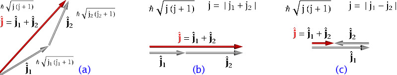
Figure 2.1. (a) The triangle rule for the addition of two angular momentum vectors showing the respective magnitudes. (b) The parallel case gives the vector with the maximum magnitude. (c) The antiparallel case gives the vector with the minimum magnitude. The range of values the quantum number j can have is |j₁ - j₂| ≤ j ≤ |j₁ + j₂|.

(a) The triangle rule for the addition of two angular momentum vectors showing the respective magnitudes. (b) The parallel case gives the vector with the maximum magnitude. (c) The antiparallel case gives the vector with the minimum magnitude. The range of values the quantum number j can have is |j1 - j2| ≤ j ≤ |j1 + j2|.

The Clebsch-Gordan coefficients are discussed in detail in most quantum mechanics textbooks (something which we leave for a future revision of this document), and tables of coefficients are readily available.

The Wigner symbols and the Racah coefficients [47][48] are defined in terms of the transformation coefficients, and therefore can also be used to perform the transformation between the uncoupled representation and the coupled representation. In the case of the addition of two angular momenta (i.e., $\hat{J} = {\hat{j}}_{1} + {\hat{j}}_{2}$ ), they are referred to as the and the Wigner 3j-symbols and the Racah V-coefficients, respectively; they are related to the Clebsch-Gordan coefficients as follows,

(2.98)

(\begin{matrix} j_{1} & j_{2} & j \\ m_{1} & m_{2} & m \end{matrix}) \equiv \frac{{(- 1)}^{j_{1} - j_{2} - m}}{\sqrt{2 j + 1}} 〈 j_{1} m_{1}, j_{2} m_{2} | j - m, j_{1} j_{2} 〉

and

(2.99)

V (j_{1} j_{2} j; m_{1} m_{2} m) \equiv \frac{{(- 1)}^{j - m}}{\sqrt{2 j + 1}} 〈 j_{1} m_{1}, j_{2} m_{2} | j - m, j_{1} j_{2} 〉 .

The Wigner 6j-symbols and the Racah W-coefficients describe the addition of three angular-momenta, $\hat{J} = {\hat{j}}_{1} + {\hat{j}}_{2} + {\hat{j}}_{3}$ , and they are defined in terms of the transformation coefficients between the decoupled representation and the coupled representation. Similarly, the Wigner 9j-symbols are defined in terms of the transformation coefficients involving the addition of four angular momenta. All of these different coefficients can be written as the sum of products of Clebsch-Gordan coefficients. Fortunately, the symmetry of the system, which is directly related to the angular momentum operators $\hat{J}, \hat{L}, and \hat{S}$ , can be used to establish whether the matrix elements of a given operator vanish or not, and therefore establish transition selection rules.

[Back to Table of Contents] [Top of Chapter 2] [scienceelearning.org]


Chapter 1. Hydrogen-like atoms.		Chapter 3. Noninteracting many-body Hamiltonians and their wavefunctions.