Chapter 7. Orbital-Dependent Functionals and Exact-Exchange Methods.
![[Note]](images/note.png) | Development note |
|---|
Development of this chapter has been temporarily delayed until the chapters covering the basics of molecular spectroscopy have been completed.
|
7.1. Introduction to very accurate density-functional methods.
As seen from our examples of density-functional theory applied to the helium atom and the hydrogen
molecule, alternative approaches are necessary to improve the accuracy
of the Kohn-Sham orbital energies.
In particular, none of the first or second generation functionals [49][182],
such as the LDA or the generalized gradient approximation (GGA) give accurate Kohn-Sham orbitals
or eigenvalues.
Because the exchange-correlation functionals are approximations in what is in principle an exact theory of electronic
structure, the resulting Kohn-Sham eigenvalues can differ significantly from what one might expect
if no approximation to the functionals was required
[174][216][178][224].
A brief summary of some of the deficiencies are described in [Koch,p.88],
most of which can be understood by comparing the exchange-correlation potential
(7.1)
v
xc
=
δ
E
xc
δ
ρ
,
resulting from the various approximations, to the results using exact methods.
Some of the requirements for the potential
v
xc
include [165]:
The asymptotic behavior of the potential should behave as
v
xc
→
-
1
r
as
r
→
∞
to cancel the Hartree self-interaction terms (e.g.
v
x
=
-
v
H
/
2
in the case of two-electron systems).
Many of the common functionals yield a potential
v
xc
with a spurious divergence at the nucleus and does not give the correct -1/r long-distance behavior
[98][104][Koch,p.88].
v
xc
should be self-interaction free, which can be expressed as follows
(7.2)
J
[
ρ
i
α
]
+
E
x
[
ρ
i
α
,
0
]
=
0
and
(7.3)
E
c
[
ρ
i
α
,
0
]
=
0
where
J[ρ] is the classical electron-electron repulsion energy which
includes the unphysical self-interaction energy
[98][Parr, p.181].
The energy eigenvalue of the highest occupied Kohn-Sham orbital
ε
N
should be exactly equal to negative of the ionization energy,
I
N
=
-
ε
N
=
E
o
N
-
1
-
E
o
N
, where
E
o
N
is the ground-state energy for a N-electron system [76][112].
For a closed subshell system,
v
xc
is a discontinuous function of the number of electrons N.
v
xc
must jump by the amount
I
N
-
A
N
as the number of electrons N is increased from
N to N-δ, where δ is an
infinitesimally small positive constant, and
A
N
=
E
o
N
-
E
o
N
+
1
is the electron affinity
[76][77].
Satisfying these conditions is critical in obtaining accurate orbitals and eigenvalues, and it is also an important first step in extending density-functional
theory to describe many different physical properties involving electronic structure. In particular,
the difference between the Kohn-Sham orbital energies provides a first
approximation to the optical excitation energies.
Several different methods have been developed to obtain exact functionals and exchange-correlation
potentials
v
xc
.
Umrigar and Gonze did one of the first studies using exact Kohn-Sham potentials
in their work on helium and two-electron ions [104]. They started with very accurate wave functions,
obtained by other methods, and then
numerically integrated these to obtain nearly exact two-electron densities. Using their
"almost exact" two-electron densities they calculated the exchange and correlation potentials,
energy densities, total energies, and compared the results to those using various LDA and GGA functionals, also calculated
using their exact two-electron densities. In this way, they were able
to identify the shortcomings of various approximate functionals. Others have used
the exact two-electron potentials
v
xc
of Umrigar and Gonze to isolate and identify deficiencies in various
functionals used in time-dependent density-functional theory (TDDFT) [216]
[224].
Both TDDFT [210][211]
[217][219][222][223][221]
[230]
and DFT perturbation theory [196][175][170][171]
are methods that provide a formal connection between the Kohn-Sham orbital
energies and excited states. For both methods
the difference between Kohn-Sham orbital energies are the zeroth order contribution to the
excitation energies, i.e.
(7.4)
ΔE
(
0
)
=
Δε
KS
=
ε
k
-
ε
j
.
Savin, Umrigar and Gonze [175][174] showed that if a very accurate exchange-correlation
potential is used, then the difference between the Kohn-Sham orbital energies,
Δε
KS
,
provides a good first
approximation to the excitation energies [174][175], as can be seen in Table 1 in the
case of the helium atom.
In fact, for the atoms studied by Filippi et al. [175],
the Kohn-Sham orbital energies always lie in between the exact singlet and triplet energy levels, with the one exception being
the
1
s
→
3
d
transition in ionized lithium.
In contrast to these exact methods,
the LDA or the generalized gradient approximation (GGA), in many cases,
will not yield any unoccupied
bound states (i.e.
ε
k
>
0
for
k
>
N
σ
), in which case Eq. (7.4) would not be valid.
For the helium atom and the hydrogen molecule, this characteristic of the unoccupied (virtual) orbitals produced by the LDA and GGA
can be seen from the output of the
first example program, freeMQM-1.cpp.
The orbital energies are stored in the array
Diag[I] and the energy of the lowest
energy virtual orbital is stored in the second element of the array, Diag[1].
For both the helium atom and the hydrogen molecule, the eigenvalue of even the lowest unoccupied orbital is greater than zero,
(7.5)
ε
2
=
Diag
[
1
]
>
0
.
What is more, in the case of helium, the LDA and the GGA give excitation energies that are
greater than the ionization energy, i.e.
(7.6)
I
=
0.903570389
a.u.
<
ε
2
-
ε
1
=
Diag
[
1
]
-
Diag
[
0
]
.
These kinds of deficiencies highlight the importance of obtaining more accurate approximations
than the LDA and the GGA.
Table 7.1. Excitation energies of He in hartree atomic units [174][175].
|
| 1s
→
2s | 23S | 0.72833 | 0.72850 | 0.7460 | 0.7232 |
| 21S | 0.75759 | 0.75775 | | 0.7687 |
|
|
| 1s
→
2p | 13P | 0.77039 | 0.77056 | 0.7772 | 0.7693 |
| 11P | 0.77972 | 0.77988 | | 0.7850 |
|
|
| 1s
→
3s | 33S | 0.83486 | 0.83504 | 0.8392 | 0.8337 |
| 31S | 0.84228 | 0.84245 | | 0.8448 |
|
|
| 1s
→
3p | 23P | 0.84547 | 0.84564 | 0.8476 | 0.8453 |
| 21P | 0.84841 | 0.84858 | | 0.8500 |
|
|
| 1s
→
3d | 13D | 0.84792 | 0.84809 | 0.8481 | 0.8481 |
| 11D | 0.84793 | 0.84809 | | 0.8482 |
|
|
| 1s
→
4s | 43S | 0.86704 | 0.86721 | 0.8688 | 0.8667 |
| 41S | 0.86997 | 0.87014 | | 0.8710 |
The last column of Table 1 shows the result of including the first order shift from Görling-Levy perturbation theory (GLPT) as
calculated by Filipi et al. [175] using their nearly exact exchange-correlation potentials.
It can be seen that the first order correction
ΔE
(
1
)
shifts singlet and triplet energies toward the experimental values.
[Back to Table of Contents] [Top of Chapter 7] [scienceelearning.org]
7.2. Many-body perturbation theory.
Before describing GLPT, it will be useful to give a brief review of the standard Rayleigh-Schrödinger (RS) time-independent perturbation
theory [Schiff, pp. 245; Sakurai, p.285; Baym, p.225; Liboff, p.549]
applied to a many-body system [Szabo, p. 320; Leach, p.114].
We seek approximate solutions to the energy eigenvalue equation
(7.7)
H
^
|
Ψ
i
〉
=
(
H
^
0
+
V
^
)
|
Ψ
i
〉
=
E
i
|
Ψ
i
〉
where the total, perturbed, Hamiltonian can be written as
(7.8)
H
^
=
H
^
0
+
V
^
.
H
^
0
is the unperturbed Hamiltonian for which
solutions are known,
(7.9)
H
^
0
|
Ψ
i
(
0
)
〉
=
E
i
(
0
)
|
Ψ
i
(
0
)
〉
and
V
^
is the perturbation, which is assumed to be small compared to
H
^
0
.
To facilitate the construction of a perturbative solution, the expansion parameter λ
is normally introduced to keep track of various orders of the perturbation.
The Hamiltonian is then written as
(7.10)
H
^
=
H
^
0
+
λ
V
^
and the perturbed wavefunction and energy levels are expanded in a power series
(7.11)
|
Ψ
i
〉
=
|
Ψ
i
(
0
)
〉
+
λ
|
Ψ
i
(
1
)
〉
+
λ
2
|
Ψ
i
(
2
)
〉
+
⋯
=
∑
n
=
0
λ
n
|
Ψ
i
(
n
)
〉
and
(7.12)
E
i
=
E
i
(
0
)
+
λE
i
(
1
)
+
λ
2
E
i
(
2
)
+
⋯
=
∑
n
=
0
λ
n
E
i
(
n
)
respectively. The value of
λ can be allowed to vary continuously from 0 to 1;
λ
=
0
corresponds to the unperturbed system and
λ
=
1
corresponds to the true, perturbed, system. In GLPT, this kind of kind
continuous variation of λ will correspond to adiabatic turning on of electron-electron
interactions.
It will prove convenient to assume that the unperturbed states are normalized,
〈
Ψ
i
(
0
)
|
Ψ
i
(
0
)
〉
=
1
, and to choose the normalization of
Ψ
i
such that
(7.13)
〈
Ψ
i
(
0
)
|
Ψ
i
〉
=
1
From Eq. (7.13), the normalization condition for
Ψ
i
leads to
(7.14)
〈
Ψ
i
(
0
)
|
Ψ
i
〉
=
1
+
∑
n
=
1
λ
n
〈
Ψ
i
(
0
)
|
Ψ
i
(
n
)
〉
=
1
which requires that
(7.15)
〈
Ψ
i
(
0
)
|
Ψ
i
(
n
)
〉
=
0
for
n
≥
1
If the power series expansions for the perturbed wavefunction,
Ψ
i
, and total energy,
E
i
, are substituted into the energy eigenvalue equation with the Hamiltonian
of Eq. (7.10), then one finds
(7.16)
(
H
^
0
+
λ
V
^
)
∑
n
=
0
λ
n
|
Ψ
i
(
n
)
〉
=
∑
m
=
0
λ
m
E
i
(
m
)
∑
n
=
0
λ
n
|
Ψ
i
(
n
)
〉
or in its expanded form
(7.17)
(
H
^
0
+
λ
V
^
)
(
|
Ψ
i
(
0
)
〉
+
λ
|
Ψ
i
(
1
)
〉+
λ
2
|
Ψ
i
(
2
)
〉
+
⋯
)
=
(
E
i
(
0
)
+
λE
i
(
1
)
+
λ
2
E
i
(
2
)
+
⋯
)
(
|
Ψ
i
(
0
)
〉
+
λ
|
Ψ
i
(
1
)
〉+
λ
2
|
Ψ
i
(
2
)
〉
+
⋯
)
Collecting terms together in powers of λ,
one can obtain the following set of equations,
(7.18)
λ
0
:
H
^
0
|
Ψ
i
(
0
)
〉
=
E
i
(
0
)
|
Ψ
i
(
0
)
〉
(7.19)
λ
1
:
H
^
0
|
Ψ
i
(
1
)
〉
+
V
^
|
Ψ
i
(
0
)
〉
=
E
i
(
0
)
|
Ψ
i
(
1
)
〉
+
E
i
(
1
)
|
Ψ
i
(
0
)
〉
(7.20)
λ
2
:
H
^
0
|
Ψ
i
(
2
)
〉
+
V
^
|
Ψ
i
(
1
)
〉
=
E
i
(
0
)
|
Ψ
i
(
2
)
〉
+
E
i
(
1
)
|
Ψ
i
(
1
)
〉
+
E
i
(
2
)
|
Ψ
i
(
0
)
〉
⋮
(7.21)
λ
n
:
H
^
0
|
Ψ
i
(
n
)
〉
+
V
^
|
Ψ
i
(
n
-
1
)
〉
=
E
i
(
0
)
|
Ψ
i
(
n
)
〉
+
E
i
(
1
)
|
Ψ
i
(
n
-
1
)
〉
+
⋯
+
E
i
(
n
)
|
Ψ
i
(
0
)
〉
By applying
〈
Ψ
i
(
0
)
|
to both sides of Eq. (7.18) and using the fact that
(7.22)
〈
Ψ
i
(
0
)
|
H
^
0
=
〈
Ψ
i
(
0
)
|
E
i
(
0
)
together with the orthogonality condition [Eq. (7.15)],
the following perturbative corrections to the energy can be obtained,
(7.23)
λ
0
:
E
i
(
0
)
=
〈
Ψ
i
(
0
)
|
H
^
0
|
Ψ
i
(
0
)
〉
(7.24)
λ
1
:
E
i
(
1
)
=
〈
Ψ
i
(
0
)
|
V
^
|
Ψ
i
(
0
)
〉
(7.25)
λ
2
:
E
i
(
2
)
=
〈
Ψ
i
(
0
)
|
V
^
|
Ψ
i
(
1
)
〉
⋮
(7.26)
λ
n
:
E
i
(
n
)
=
〈
Ψ
i
(
0
)
|
V
^
|
Ψ
i
(
n
-
1
)
〉
The first order energy correction,
E
i
(
1
)
,
is expressed in terms of the known
unperturbed quantities
E
i
(
0
)
and
Ψ
i
(
0
)
,
but the higher order energy corrections also need to be expressed in terms of the
unperturbed quantities.
To achieve this, we expand the perturbative corrections to the wavefunctions,
|
Ψ
i
(
n
)
〉
,
in the complete set of eigenstates of
H
^
0
,
(7.27)
|
Ψ
i
(
n
)
〉
=
∑
k
'
|
Ψ
k
(
0
)
〉
〈
Ψ
k
(
0
)
|
Ψ
i
(
n
)
〉
Using this expansion, we can begin to calculate the higher order corrections to the energy.
For example, by substituting the expansion with n=1 into the expression for
the second order energy correction we have
(7.28)
E
i
(
2
)
=
〈
Ψ
i
(
0
)
|
V
^
|
Ψ
i
(
1
)
〉
=
∑
k
'
〈
Ψ
i
(
0
)
|
V
^
|
Ψ
k
(
0
)
〉
〈
Ψ
k
(
0
)
|
Ψ
i
(
1
)
〉
were the prime means that
k
=
i
has been excluded from the summation.
The last term in Eq. (7.28),
〈
Ψ
k
(
0
)
|
Ψ
i
(
1
)
〉
,
can be obtained by applying
〈
Ψ
k
(
0
)
|
to both sides of Eq. (7.21)
(7.29)
〈
Ψ
k
(
0
)
|
H
^
0
|
Ψ
i
(
n
)
〉
+
〈
Ψ
k
(
0
)
|
V
^
|
Ψ
i
(
n
-
1
)
〉
=
E
i
(
0
)
〈
Ψ
k
(
0
)
|
Ψ
i
(
n
)
〉
+
E
i
(
1
)
〈
Ψ
k
(
0
)
|
Ψ
i
(
n
-
1
)
〉
+
⋯
+
E
i
(
n
)
〈
Ψ
k
(
0
)
|
Ψ
i
(
0
)
〉
Using again the eigenvalue relation
(7.30)
〈
Ψ
k
(
0
)
|
H
^
0
=
〈
Ψ
k
(
0
)
|
E
k
(
0
)
we can rewrite Eq. (7.29) as
(7.31)
(
E
i
(
0
)
-
E
k
(
0
)
)
〈
Ψ
k
(
0
)
|
Ψ
i
(
n
)
〉
=
(
〈
Ψ
k
(
0
)
|
V
^
|
Ψ
i
(
n
-
1
)
〉
-
E
i
(
1
)
〈
Ψ
k
(
0
)
|
Ψ
i
(
n
-
1
)
〉
-
⋯
-
E
i
(
n
)
〈
Ψ
k
(
0
)
|
Ψ
i
(
0
)
〉
)
If we assume that
k
≠
i
then we can use the fact that the
|
Ψ
i
(
n
)
〉
are orthogonal and drop the last term in Eq. (7.31) and write
(7.32)
〈
Ψ
k
(
0
)
|
Ψ
i
(
n
)
〉
=
1
E
i
(
0
)
-
E
k
(
0
)
(
〈
Ψ
k
(
0
)
|
V
^
|
Ψ
i
(
n
-
1
)
〉
-
E
i
(
1
)
〈
Ψ
k
(
0
)
|
Ψ
i
(
n
-
1
)
〉
-
E
i
(
2
)
〈
Ψ
k
(
0
)
|
Ψ
i
(
n
-
2
)
〉
-
⋯
)
By setting n = 1 in the previous equation, we obtain the first order correction
to the wavefunction,
(7.33)
〈
Ψ
k
(
0
)
|
Ψ
i
(
1
)
〉
=
〈
Ψ
k
(
0
)
|
V
^
|
Ψ
i
(
0
)
〉
E
i
(
0
)
-
E
k
(
0
)
Substituting this result into the equation for the second order energy correction
[Eq. (7.25)] we have
(7.34)
E
i
(
2
)
=
∑
k
'
|
〈
Ψ
k
(
0
)
|
V
^
|
Ψ
i
(
0
)
〉
|
2
E
i
(
0
)
-
E
k
(
0
)
The other higher order corrections can also be obtained by following this kind of procedure, one by one.
At this point, we will discuss the meaning of the unperturbed excited states
|
Ψ
i
(
0
)
〉
(n≠0) used in the perturbation expansions.
In previous sections, we have only managed to develop approximate
solutions to the unperturbed ground state, which were Slater determinants built
from single-particle spin-orbitals. In short-hand notation these are given by
[Szabo, pp.58, 303, 341; Levine, p.512]
(7.35)
|
Ψ
0
(
0
)
〉
=
|
χ
1
χ
2
⋯χ
a
χ
b
⋯χ
N
〉
An individual spin-orbital with explicit spin dependence can be written as
(7.36)
χ
(
x
)
=
ϕ
σ
(
r
)
=
{
ϕ
(
r
)
α
for
σ
=
↑
ϕ
(
r
)
β
for
σ
=
↓
and the N spin-orbitals incorporated into the determinant will have the form
(7.37)
χ
1
(
x
1
)
=
ϕ
1↑
(
r
1
)
=
ϕ
1
(
r
1
)
α
(
σ
1
)
χ
2
(
r
2
)
=
ϕ
1↓
(
r
2
)
=
ϕ
1
(
x
2
)
β
(
σ
2
)
χ
3
(
x
3
)
=
ϕ
2↑
(
r
3
)
=
ϕ
2
(
r
3
)
α
(
σ
3
)
χ
4
(
x
4
)
≐
ϕ
2↓
(
r
4
)
=
ϕ
2
(
r
4
)
β
(
σ
4
)
⋮
where
ϕ
(
r
)
is the spatial part of the spin-orbital.
The expansion of the molecular orbitals
with K spatial basis functions [Eq. (5.45)] results in 2K
spin-orbitals. For a N-electron system, 2K-N of these spin-orbitals
will be unoccupied (virtual) orbitals. The excited states
|
Ψ
i
(
0
)
〉
,
constructed from spin-orbitals, will include contributions from determinants in which electrons
have been excited from the occupied ground state orbitals to virtual orbitals.
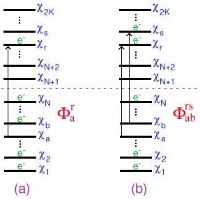
A singly excited determinant, for example, can be written as
|
Ψ
a
r
〉
=
|
χ
1
χ
2
⋯χ
r
χ
b
⋯χ
N
〉
,
which corresponds to an electron being excited from an occupied spin-orbital
χ
a
to a virtual orbital
χ
r
,
as illustrated in Figure 1(a). Similarly, a doubly excited determinant
can be written as
|
Ψ
ab
rs
〉
=
|
χ
1
χ
2
⋯χ
r
χ
s
⋯χ
N
〉
,
which corresponds to electrons being excited from the spin-orbitals
χ
a
and
χ
b
to the virtual orbitals
χ
r
and
χ
s
[Fig. 1(b)]. It is important to keep in mind that
even for the ground state, the single Slater determinant
|
χ
1
χ
2
⋯χ
a
χ
b
⋯χ
N
〉
will be an exact solution only
for systems of independent electrons (noninteracting with each other), with only single-particle interactions
[Szabo, p. 130]. This would include systems in which a many-body
interaction has been transformed into an effective one-body interaction.
In general, both the ground state and the excited states obtained from these systems,
|
Ψ
a
r
〉
,
|
Ψ
ab
rs
〉
,
|
Ψ
abc
rst
〉
,
etc., will only be approximations to the exact states,
|
Ψ
i
〉
. Nevertheless, the Slater determinants, which serve as exact solutions
in the independent-electron approach, can be used to construct the exact excited states.
[Back to Table of Contents] [Top of Chapter 7] [scienceelearning.org]
7.3. Møller-Plesset perturbation theory (MPPT).
As our first example of many-body perturbation theory, we will let the unperturbed Hamiltonian
be given by the Fock operator [Eq. (5.41)]
(7.38)
H
^
0
=
∑
i
=
1
N
ℱ
^
(
i
)
=
∑
i
=
1
N
[
ℋ
core
(
i
)
+
v
^
HF
(
i
)
]
.
The perturbation is
(7.39)
V
^
=
H
^
-
H
^
0
=
V
^
ee
-
V
^
HF
,
where the total Hamiltonian,
H
^
, is given by Eq. (5.3)
[and Eq. (6.1)] and as before
V
^
ee
is given by
(7.40)
V
^
ee
=
∑
i
<
j
N
1
r
ij
The Hartree-Fock potential operator,
V
^
HF
,
is obtained from the Coulomb and exchange terms of the Fock operator
[Eq. (5.41)]
(7.41)
V
^
HF
=
∑
i
=
1
N
∑
j
=
1
N
[
𝒥
j
(
i
)
-
𝒦
j
(
i
)
]
=
∑
i
=
1
N
v
^
HF
(
i
)
,
where
v
^
HF
(
i
)
is defined as the Hartree-Fock potential operator of the ith electronl. and
H
^
=
H
^
0
+
V
^
is equal to the Hamiltonian operator in Eq. (5.3).
Since, in this example,
H
^
0
is a single-particle operator we can use
Eq. (5.13) together with the definition of the orbital energies [Eq. (5.43)]
to obtain
(7.42)
E
0
(
0
)
=
〈
Ψ
0
(
0
)
|
H
^
0
|
Ψ
0
(
0
)
〉
=
〈
χ
1
χ
2
⋯χ
a
χ
b
⋯χ
N
|
H
^
0
|
χ
1
χ
2
⋯χ
a
χ
b
⋯χ
N
〉
=
∑
i
=
1
N
ε
i
Similarly, the zeroth order contribution to an excited state is
(7.43)
E
a
r
(
0
)
=
〈
Ψ
a
r
|
H
^
0
|
Ψ
a
r
〉
=
〈
χ
1
χ
2
⋯χ
r
χ
b
⋯χ
N
|
H
^
0
|
χ
1
χ
2
⋯χ
r
χ
b
⋯χ
N
〉
=
∑
i
=
1
N
ε
i
+
ε
r
-
ε
a
The difference between the two is the zeroth order excitation energy
(7.44)
ΔE
a
r
(
0
)
≡
E
a
r
(
0
)
-
E
0
(
0
)
=
ε
r
-
ε
a
From Eq. (7.24) we know that the first order correction to the energy is given by
(7.45)
E
0
(
1
)
=
〈
Ψ
0
(
0
)
|
V
^
|
Ψ
0
(
0
)
〉
=
〈
Ψ
0
(
0
)
|
V
^
ee
-
V
^
HF
|
Ψ
0
(
0
)
〉
To calculate the first order correction
E
0
(
1
)
,
we will first calculate
〈
Ψ
0
(
0
)
|
V
^
ee
|
Ψ
0
(
0
)
〉
and
〈
Ψ
0
(
0
)
|
V
^
HF
|
Ψ
0
(
0
)
〉
separately and then take the difference. The contribution from
V
^
ee
was calculated before in Section 5.1
[Eq. (5.15), Eq. (5.19), and Eq. (5.20)] using
Eq. (5.14), which we repeat here for clarity,
(7.46)
〈
Ψ
0
(
0
)
|
V
^
ee
|
Ψ
0
(
0
)
〉
=
1
2
∑
i
≠
j
N
〈
χ
1
χ
2
⋯χ
a
χ
b
⋯χ
N
|
1
r
ij
|
χ
1
χ
2
⋯χ
a
χ
b
⋯χ
N
〉
=
1
2
∑
i
,
j
N
[
〈
χ
i
χ
j
|
1
r
12
|
χ
i
χ
j
〉
-
〈
χ
i
χ
j
|
1
r
12
|
χ
j
χ
i
〉
]
=
1
2
∑
i
,
j
N
〈
χ
i
|
[
𝒥
j
(
x
1
)
-
𝒦
j
(
x
1
)
]
|
χ
i
〉
=
1
2
∑
i
=
1
N
〈
χ
i
|
v
^
HF
|
χ
i
〉
=
1
2
∑
i
,
j
N
[
J
ij
-
K
ij
]
where
(7.47)
J
ij
=
〈
χ
i
|
𝒥
j
(
x
1
)
|
χ
i
〉
=
〈
χ
i
χ
j
|
1
r
12
|
χ
i
χ
j
〉
and
K
ij
=
〈
χ
i
|
𝒦
j
(
x
1
)
|
χ
i
〉
=
〈
χ
i
χ
j
|
1
r
12
|
χ
j
χ
i
〉
Similarly, the contribution to the first order energy correction from
V
^
HF
can be calculated using Eq. (5.13),
(7.48)
〈
Ψ
0
(
0
)
|
V
^
HF
|
Ψ
0
(
0
)
〉
=
〈
χ
1
χ
2
⋯χ
a
χ
b
⋯χ
N
|
∑
i
=
1
N
v
^
HF
(
i
)
|
χ
1
χ
2
⋯χ
a
χ
b
⋯χ
N
〉
=
∑
i
=
1
N
〈
χ
i
|
v
^
HF
|
χ
i
〉
=
∑
i
,
j
N
[
J
ij
-
K
ij
]
.
The first order perturbation correction can then be written as
(7.49)
E
0
(
1
)
=
〈
Ψ
0
(
0
)
|
V
^
ee
-
V
^
HF
|
Ψ
0
(
0
)
〉
=
-
1
2
∑
i
=
1
N
〈
χ
i
|
v
^
HF
|
χ
i
〉
=
-
1
2
∑
i
,
j
N
[
J
ij
-
K
ij
]
.
Combining the zeroth order and first order terms gives us
(7.50)
E
=
E
0
(
0
)
+
E
0
(
1
)
=
∑
i
=
1
N
ε
i
-
1
2
∑
i
,
j
N
[
J
ij
-
K
ij
]
,
which is the same result as was found in Section 5.2 [Eq. (5.44)].
The first order correction to an excited state can be obtained from Eq. (7.49) by replacing an
orbital from the ground state,
χ
a
,
with a virtual orbital,
χ
r
,
(7.51)
E
a
r
(
1
)
=
〈
Ψ
a
r
|
V
^
ee
-
V
^
HF
|
Ψ
a
r
〉
=
-
1
2
∑
i
,
j
N
[
J
ij
-
K
ij
]
-
∑
i
=
1
N
[
J
ir
-
K
ir
]
+
∑
i
=
1
N
[
J
ia
-
K
ia
]
+
[
J
ar
-
K
ar
]
=
-
1
2
∑
i
=
1
N
〈
χ
i
|
v
^
HF
|
χ
i
〉
-
〈
χ
r
|
v
^
HF
|
χ
r
〉
+
〈
χ
a
|
v
^
HF
|
χ
a
〉
+
[
J
ar
-
K
ar
]
.
The difference between
E
a
r
(
1
)
and
E
0
(
1
)
is the first order contribution to the excitation energy
(7.52)
ΔE
a
r
(
1
)
≡
E
a
r
(
1
)
-
E
0
(
1
)
=
-
〈
χ
r
|
v
^
HF
|
χ
r
〉
+
〈
χ
a
|
v
^
HF
|
χ
a
〉
+
[
J
ar
-
K
ar
]
[Back to Table of Contents] [Top of Chapter 7] [scienceelearning.org]
7.4. Görling-Levy perturbation theory (GLPT).
In a future revsion of this document, we will see that in the GLPT approach, an adiabatic connection parameter α is treated
as the expansion parameter in perturbation theory [196].
We will also see in TDDFT, that the Kohn-Sham levels are split and shifted toward their true values by contributions from the time-dependent xc kernel in the linear-response regime, where the xc kernel is
(7.53)
f
xc
(
r
,
r′
,
t
-
t′
)
=
δv
xc
(
r
,
t
)
δρ
(
r′
,
t′
)
.
An accurate calculation of the exchange-correlation potential
v
xc
will still be at least as important as an accurate calculation of
f
xc
in TDDFT [216].
| |
|---|
| ...to be continued. |
[Back to Table of Contents] [Top of Chapter 7] [scienceelearning.org]
7.5. The Optimized Effective Potential Method (OEP).
In a future revision of this document, we will also show how the optimized effective potential method provides a procedure to transform the nonlocal Hartree-Fock (HF) exchange operator into a local variationally optimized exchange potential that can be incorporated
into Kohn-Sham density-functional calculations. Sharp and Horton [152]
and Talman and Shadwick [153] used variational principles [152]
[153] in the original development of the
OEP integrodifferential equations. Other methods have been used to derive the OEP equations which do not require any discussion
of the optimized exchange potential method itself [171][164][78].
Görling and Levy, for example, have derived the OEP equations using perturbation theory
[171][170] and Shaginyan
used linear-response theory [164].
It was explained by Sahni, Gruenebaum, and Perdew [154] and Perdew and Norman [155]
that the Talman-Shadwick energy-optimized local potential is “an exact
realization of the Kohn-Sham potential for ‘exchange only’ in atoms” and that the
only difference between the exchange-only Kohn-Sham and Hartree-Fock theories is that the Hartree-Fock
effective potential is nonlocal.
Application of the OEP in its original form is computationally demanding, which has limited its
application to a few simple systems [153][156][182].
Krieger, Li, and Iarafe, however, presented an approximation that helped revitalize interest in
the method [159]
[160][161][162][163][165].
Kim et al. [178] have implemented
the Krieger-Li-Iafrate (KLI) approximation to the optimized effective potential (OEP) exact exchange functional to study small molecules,
using a three-dimensional (3D) finite-difference pseudopotential method [117] [118].
They found that the addition of LDA or GGA correlation functions did not lead
to systematic improvements over the KLI exchange-only approximation. It has been shown by
Vasilev et al. [220], however, and further explained by Burke et al. [224], that in
TDDFT the correlation effects are more important than in calculations of the time-independent ground state properties. In particular, an antiparallel spin correlation functional
f
xc
↑↓
contributes to the splitting of the Kohn-Sham energy eigenvalues [224].
| |
|---|
| ...to be continued. |
[Back to Table of Contents] [Top of Chapter 7] [scienceelearning.org]