4.1. Orbital angular momentum in many-electron atoms.
If
Ψ
is a simultaneous many-body eigenstate of a set of operators, then all of operators in the set
must commute with each other. In the case of the total
angular momentum operators, this requirement resulted in the two representations shown in
Eqs. (2.89) and (2.92). Ideally, we would like to construct a solution of the Schrödinger equation
Ψ
to be not only an eigenstate of the Hamiltonian operator,
H
^
,
but also of the angular momentum operators in the coupled representation. In practice, this may be
impractical and unnecessary, as much about a system can be learned from the symmetry properties alone.
Even in the case of atoms, finding a set of commuting operators inevitably
involves some level of approximation. Case and point being the Dirac equation describing a particle
in a central field―to which the Schrödinger equation is an approximation. The relativistic Hamiltonian operator can be written as
(4.1)
H
^
=
c
α
^
·
p
+
β
^
mc
2
+
V
(
r
)
where
(4.2)
β
^
=
(
1
0
0
-
1
)
and
(4.3)
α
^
i
=
(
0
σ
^
i
σ
^
i
0
)
;
Both
β
^
and
α
^
are 4×4 dimensional matrices, and
σ
^
are the 2×2 dimensional Pauli spin matrices [Eq. (2.21)].
Even for a free particle without the central field term,
V
(
r
)
,
the orbital angular momentum,
L
^
,
is not a constant of the motion [Sakurai67, p.113], in fact,
(4.4)
[
H
^
,
L
^
i
]
=
-
iℏc
(
α
^
×
p
)
i
where i = x, y, z.
Similarly, for the spin operator we have
(4.5)
[
H
^
,
Σ
^
i
]
=
i2c
(
α
^
×
p
)
i
with i = x, y, z,
and
(4.6)
S
^
=
ℏ
2
Σ
^
=
ℏ
2
(
σ
^
0
0
σ
^
)
.
Without the central-field term,
V
(
r
)
,
we could choose a frame of reference in which the particle is at rest and, therefore,
(4.7)
[
H
^
,
L
^
i
]
=
[
H
^
,
Σ
^
i
]
=
0
;
In the nonrelativistic limit, this will still be a good approximation, even with the central-field potential.
On the other hand, we can see from the previous equations that the total angular momentum of a single-particle in a spherically symmetric central potential
is a constant of the motion
(4.8)
[
H
^
,
J
^
i
]
=
[
H
^
,
L
^
i
+
S
^
i
]
=
[
H
^
,
L
^
i
]
+
[
H
^
,
ℏ
2
Σ
^
i
]
=
-
iℏc
(
α
^
×
p
)
i
+
iℏc
(
α
^
×
p
)
i
=
0
where we have used
(4.9)
J
^
=
L
^
+
S
^
=
L
^
+
ℏ
2
Σ
^
.
Hence a set of commuting observables do exist for a relativistic particle; they are
H
^
,
J
^
2
,
J
^
z
, and
Κ
^
,
where the operator
Κ
^
is given by
[Schiff,p.483; Sakurai,p.123; Baym,p.565]
(4.10)
Κ
^
=
β
^
(
ℏ
+
Σ
^
·
L
^
)
.
The operator
Κ
^
commutes with the relativistic Hamiltonian and the total momentum operator,
J
^
,
and
κ
is a good quantum number.
Κ
^
and it's quantum number,
κ
,
describe the extent that the spin and orbital momentum are aligned.
We will return later to discuss the Schrödinger equation as an approximation to Dirac equation, but
for the moment we will just mention the fact that many terms that can be included in the Schrödinger equation
are actually derived from the Dirac equation, with the spin-orbit interaction being a prime example.
In the nonrelativistic limit, the Dirac equation describing a single electron in a central field, given by the Coulomb potential,
V
(
r
)
=
-
Z
/
r
,
will reduce to the Schrödinger equation for hydrogen-like atoms, and in this case the total
orbital angular momentum is a constant of the motion. The Cartesian components of the orbital angular momentum operator,
L
^
=
r
×
p
,
in the position-space representation are given by the following differential operators
(4.11)
L
^
x
=
-
iℏ
(
y
∂
∂
z
-
z
∂
∂
y
)
=
iℏ
(
sinφ
∂
∂
θ
+
cotθ
cosφ
∂
∂
φ
)
(4.12)
L
^
y
=
-
iℏ
(
z
∂
∂
x
-
x
∂
∂
z
)
=
iℏ
(
-
cosφ
∂
∂
θ
+
cotθ
sinφ
∂
∂
φ
)
(4.13)
L
^
z
=
-
iℏ
(
x
∂
∂
y
-
y
∂
∂
x
)
=
-
iℏ
∂
∂
φ
(4.14)
L
^
2
=
L
^
x
2
+
L
^
y
2
+
L
^
z
2
=
-
ℏ
2
[
1
sin
2
θ
∂
2
∂
φ
2
+
1
sinθ
(
∂
∂
θ
sinθ
∂
∂
θ
)
]
and we have also shown the operators in spherical coordinates; As a reminder the two coordinate systems
are related by
(4.15)
x
=
r
cosφ
sinθ
y
=
r
sinφ
sinθ
z
=
r
cosθ
.
The spherical harmonics,
Y
l
m
l
(
θ
,
φ
)
,
are the simultaneous eigenfunctions of
L
^
2
and
L
^
z
,
the application of which leads to the following eigenvalue equations
(4.16)
L
^
2
Y
l
m
l
(
θ
,
φ
)
=
ℏ
2
l
(
l
+
1
)
Y
l
m
l
(
θ
,
φ
)
and
(4.17)
L
^
z
Y
l
m
l
(
θ
,
φ
)
=
ℏ
m
l
Y
l
m
l
(
θ
,
φ
)
.
We will attempt to follow international convention [see Appendix A], in which
case the operators
L
^
2
and
L
^
z
,
and their quantum numbers for atoms,
L
and
M
L
,
describe the total system, not individual electrons, which use the lower case letters for the quantum numbers,
l
and
m
l
.
The operators
L
^
,
S
^
,
and
J
^
are equal to the vector sum of the single-particle operators
l
^
i
,
s
^
i
, and
j
^
i
, i.e.,
(4.18)
L
^
=
∑
i
=
1
N
l
^
i
,
S
^
=
∑
i
=
1
N
s
^
i
,
and
J
^
=
∑
i
=
1
N
j
^
i
,
respectively.
For a many-electron atomic Hamiltonian that neglects electron-electron interactions, that is,
for a fictitious system of independent electrons described by
Eqs. (3.1)-(3.4), we can write the atomic orbitals as
ψ
i
(
r
i
)
=
ψ
n
i
l
i
m
li
(
r
i
,
θ
i
,
φ
i
)
for each electron. Neglecting electron-electron interactions also allows us to write the following orbital angular momentum eigenvalue equations,
(4.19)
l
^
i
2
ψ
n
i
l
i
m
li
(
r
i
,
θ
i
,
φ
i
)
=
ℏ
2
l
i
(
l
i
+
1
)
ψ
n
i
l
i
m
li
(
r
i
,
θ
i
,
φ
i
)
and
(4.20)
l
^
iz
ψ
n
i
l
i
m
li
(
r
i
,
θ
i
,
φ
i
)
=
ℏ
m
li
ψ
n
i
l
i
m
li
(
r
i
,
θ
i
,
φ
i
)
.
The solutions are the hydrogen-like wavefunctions,
(4.21)
ψ
i
(
r
i
)
=
ψ
n
i
l
i
m
li
(
r
i
,
θ
i
,
φ
i
)
=
R
n
i
l
i
(
r
i
)
Y
l
i
m
li
(
θ
i
,
φ
i
)
,
where
n
i
,
l
i
, and
m
l
i
are the principle quantum number and orbital angular momentum quantum numbers
of the ith electron, respectively. As we will show in what follows, only
if the electron-electron interactions are neglected will
(4.22)
[
l
^
i
2
,
H
^
]
=
[
l
^
iz
,
H
^
]
=
0
;
However, if the
V
^
ee
term is included in the Hamiltonian, then
(4.23)
[
l
^
i
2
,
H
^
]
≠
0
,
[
l
^
iz
,
H
^
]
≠
0
,
and the hydrogen-like wavefunctions will be useful in constructing only approximate many-electron wavefunctions.
Nevertheless, because of the spherical symmetry of atoms, the
total orbital angular momentum, in the nonrelativistic limit, is a constant
of the motion [also see Bernath, pp. 131-132],
(4.24)
[
L
^
2
,
H
^
]
=
[
L
^
z
,
H
^
]
=
0
,
even with the
V
^
ee
term. To show this we would first like to establish that
[
l
^
iz
,
H
^
]
≠
0
,
which will be true if
l
^
iz
V
^
ee
≠
0
, as can be verified by applying the commutator to an arbitrary function of position.
To calculate
l
^
iz
V
^
ee
we will use the fact that
(4.25)
l
^
iz
(
1
r
ij
)
=
-
iℏ
(
x
i
∂
∂
y
i
-
y
i
∂
∂
x
i
)
(
1
r
ij
)
=
iℏ
(
x
i
y
i
-
y
j
r
ij
3
-
y
i
x
i
-
x
j
r
ij
3
)
=
iℏ
(
x
j
y
i
-
x
i
y
j
r
ij
3
)
,
where the z-component of single-particle orbital angular momentum operator is given by
(4.26)
l
^
iz
=
-
iℏ
(
x
i
∂
∂
y
i
-
y
i
∂
∂
x
i
)
and we have used the following derivatives
(4.27)
∂
∂
x
i
(
1
r
ij
)
=
-
x
i
-
x
j
r
ij
3
,
∂
∂
y
i
(
1
r
ij
)
=
-
y
i
-
y
j
r
ij
3
,
and
r
ij
=
(
x
i
-
x
j
)
2
+
(
y
i
-
y
j
)
2
+
(
z
i
-
z
j
)
2
.
Replacing
r
ij
-
1
in Eq. (4.25) with the operator
V
^
ee
leads to
(4.28)
l
^
iz
V
^
ee
=
-
iℏ
(
x
i
∂
∂
y
i
-
y
i
∂
∂
x
i
)
(
1
2
∑
i
=
1
N
∑
j
≠
i
N
1
r
ij
)
=
iℏ
∑
j
≠
i
N
x
j
y
i
-
x
i
y
j
r
ij
3
,
which is equal to the following commutator of the single-electron orbital angular momentum operator and the Hamiltonian operator
(4.29)
[
l
^
iz
,
H
^
]
=
[
l
^
iz
,
V
^
ee
]
=
iℏ
∑
j
≠
i
N
x
j
y
i
-
x
i
y
j
r
ij
3
,
and for clarity we repeat here the expression for the electron-electron interaction energy (in atomic units)
(4.30)
V
^
ee
=
∑
i
<
j
N
1
r
ij
=
1
2
∑
i
=
1
N
∑
j
≠
i
N
1
r
ij
.
So, in fact, we see from Eq. (4.29) that when electron-electron interactions are included in the Hamiltonian
of a many-electron atom
[
l
^
iz
,
H
^
]
≠
0
.
As mentioned previously, the total orbital angular momentum,
L
^
,
is a different story because of the overall spherical symmetry of atoms, and because
(4.31)
L
^
z
V
^
ee
=
∑
i
=
1
N
l
^
iz
V
^
ee
=
iℏ
∑
i
=
1
N
∑
j
≠
i
N
x
j
y
i
-
x
i
y
j
r
ij
3
=
0
;
Eq. (4.31) is equal to the commutator of the total orbital angular momentum operator and the Hamiltonian operator
(4.32)
[
L
^
z
,
H
^
]
=
[
L
^
z
,
V
^
ee
]
=
0
.
Moreover, the spherical symmetry of atoms means that the direction of the z-axis is an arbitrary choice and
therefore it must also be true that
(4.33)
[
L
^
x
,
H
^
]
=
[
L
^
y
,
H
^
]
=
[
L
^
z
,
H
^
]
=
0
,
from which it follows
(4.34)
[
L
^
x
2
,
H
^
]
=
[
L
^
y
2
,
H
^
]
=
[
L
^
z
2
,
H
^
]
=
0
,
and this finally leads us to
(4.35)
[
L
^
2
,
H
^
]
=
0
.
The single-electron orbital angular momentum eigenvalue equations were given in Eqs. (4.19) and (4.20). Similarly, the total orbital angular momentum eigenvalue equations of multi-electron atoms are
(4.36)
L
^
2
Ψ
=
ℏ
2
L
(
L
+
1
)
Ψ
and
(4.37)
L
^
z
Ψ
=
ℏM
L
Ψ
.
To understand the relationship between the total orbital-angular momentum,
L
^
,
and the orbital angular momentum of the individual electrons,
l
^
i
,
one could imagine starting with a noninteracting Hamiltonian and
then adiabatically turning on the electron-electron interactions. As we have shown, without
the electron-electron interactions both
L
^
and
l
^
i
are constants of the motion and the values of
l
^
i
obviously determine the possible values of
L
^
. As the electron-electron interactions are adiabatically turned on, the individual momenta
l
^
i
are no longer "good", but the total orbital-angular momentum,
L
^
,
is not affected. In other words, even with electron-electron interactions we can still use the single-electron
quantum numbers
l
i
and
m
l
i
to determine the possible values of
L
and
M
L
.
It can be shown, for example, that for the addition of two angular momenta
(4.38)
L
^
=
l
^
1
+
l
^
2
the possible values of L are
(4.39)
L
=
l
1
+
l
2
,
l
1
+
l
2
-
1
,
…
,
|
l
1
-
l
2
|
.
For N-electrons we can iterate this process by first combining the l
values for two electrons, as was done above [Liboff, pp. 354-355]
(4.40)
l
'
=
l
1
+
l
2
,
…
,
❘
l
1
-
l
2
❘
then combining the
l
'
values with those of the third electron
(4.41)
l
''
=
l
'
+
l
3
,
…
,
|
l
'
-
l
3
|
and similarly for the fourth electron
(4.42)
l
'''
=
l
''
+
l
4
,
…
,
|
l
''
-
l
4
|
.
Finally, for N-electrons we have
(4.43)
L
=
l
max
,
l
max
-
1
,
…
,
|
l
min
|
where
(4.44)
l
max
=
∑
i
=
1
N
l
i
(4.45)
l
min
=
{
l
N
-
∑
i
=
1
N
-
1
l
i
if
l
N
-
∑
i
=
1
N
-
1
l
i
>
0
0
if
l
N
-
∑
i
=
1
N
-
1
l
i
≤
0
and in the expression for
l
min
we have chosen the last electron such that it has the largest l value, i.e.,
l
N
≥
l
i
for all i. By analogy to the spectroscopic notation used to describe the single-electron
orbitals of the hydrogen atom, s, p, d, f,...(sharp, principle, diffuse,...) for l = 0, 1, 2, 3...,
many-electron atoms use capital letters, S, P, D, F,... for L = 0, 1, 2, 3...
The notation used to describe the orbital angular momentum quantum numbers for atoms and diatomic molecules
is summarized below in Table 1. We will only mention at this point that because molecules are not spherically
symmetric,
[
L
^
2
,
H
^
]
≠
0
.
However, for diatomic molecules
[
L
^
z
,
H
^
]
≠
0
,
and the projection of orbital angular momentum onto the interatomic axis is still a good quantum number.
Table 4.1. Orbital angular momentum quantum numbers and symbols used to describe atoms and molecules.
|
Quantum Number
1
2
3
4
5
6
One-electron atoms
l
s
p
d
f
g
h
One-electron atoms: Z'-projection
m
l
Multi-electron atoms
L
S
P
D
F
G
H
Multi-electron atoms: Z'-projection
M
L
Diatomic molecules: single-electron 𝓏-projection
λ
i
σ
π
δ
ϕ
γ
η
Diatomic molecules: total 𝓏-projection
Λ
=
∑
i
=
1
N
λ
i
Σ
Π
Δ
Φ
Γ
Η
|
In Equations (4.4)-(4.8), we showed that
H
^
,
J
^
2
,
J
^
z
, and
Κ
^
is a set of commuting observables for relativistic electrons in a central field. In the nonrelativistic limit, when the Dirac
equation reduces to Schrödinger equation, and if there is a negligible contribution from the spin-orbit interaction energy, then
{
H
^
,
L
^
2
,
L
^
z
,
S
^
2
,
S
^
z
}
, or
{
H
^
,
J
^
2
,
J
^
z
,
L
^
2
,
S
^
2
}
form a set of commuting observables.
An atomic energy level can be labeled with the term symbol
(4.46)
Multiplicity
→
2
S
+
1
L
↓
J
←
Level
Orbital
angular
momentum
Without spin dependent terms in the Hamiltonian, however,
2
S
+
1
L
J
does not label a distinct atomic state or energy level. For given values of the quantum numbers L and S, the possible eigenvalues of the angular momentum operators
L
^
z
and
S
^
z
are given by
ℏM
L
=
-
ℏL
,
-
ℏ
(
L
+
1
)
,
…
,
ℏ
(
L
-
1
)
,
ℏL
,
and
ℏM
S
=
-
ℏS
,
-
ℏ
(
S
+
1
)
,
…
,
ℏ
(
S
-
1
)
,
ℏS
, respectively. Thus, without any spin dependent terms in the Hamiltonian, the degeneracy of the energy level
is (2L + 1)(2S + 1), and therefore, in general, the angular momentum quantum numbers do not correspond to distinct energy eigenvalues. Similarly, term symbols for diatomic molecules can be written as
(4.47)
Multiplicity
→
2
S
+
1
Λ
↓
Ω
←
Quantum number of
J
^
az
Quantum number of
L
^
z
,
which will be discussed in detail later.
[Back to Table of Contents] [Top of Chapter 4] [scienceelearning.org]
4.2. Slater determinants as spin angular momentum eigenstates.
Constructing a symmetric or antisymmetric state using a linear combination of base kets from the decoupled
representation [Eq. (2.88)] will not necessarily produce an eigenstate of the angular momentum
operators. This means that a single Slater determinant will not be sufficient to construct an eigenstate with the same symmetry properties of
the exact wavefunction. In Eqs. (4.25)-(4.29) we showed that if electron-electron interactions are included in the Hamiltonian, then
[
l
^
iz
,
H
^
]
≠
0
.
In the case of spin angular momentum, however,
[
s
^
iz
,
H
^
]
=
0
,
unless there is a spin dependent term in the Hamiltonian. In general, Slater determinants will not be eigenstates of single-electron
spin operators, as can be seen applying
s
^
iz
to the wavefunction in Eq. (3.43)
(4.48)
s
^
1z
Ψ
(
x
1
,
x
2
,
…
,
x
N
)
=
s
^
1z
1
N
!
∑
j
,
k
,
l
,
⋯
N
ε
jkl⋯
χ
j
(
x
1
)
χ
k
(
x
2
)
χ
l
(
x
3
)
⋯
=
1
N
!
∑
j
,
k
,
l
,
⋯
N
ε
jkl⋯
s
^
1z
χ
j
(
x
1
)
χ
k
(
x
2
)
χ
l
(
x
3
)
⋯
=
(
ℏ
2
)
1
N
!
∑
j
,
k
,
l
,
⋯
N
ε
jkl⋯
(
-
1
)
j
+
1
χ
j
(
x
1
)
χ
k
(
x
2
)
χ
l
(
x
3
)
⋯
In Eq. (4.48) we have assumed that j odd labels a spin-orbital occupied by an electron with its spin-up, and j even labels an orbital occupied by an electron with its spin-down. This convention allows us to write
(4.49)
s
^
1
z
χ
j
(
x
1
)
=
±
ℏ
2
χ
j
(
x
1
)
where the plus sign is for j odd, the minus sign is for j even. The choice of i = 1 as an example in Eqs. (4.48) and (4.49) was arbitrary. It has also been assumed that the spin-orbitals are as defined in Eq. (3.28).
From Eq. (4.48) it can be seen that for the many-electron wavefunction
(
Ψ
)
to be an eigenstate of
s
^
iz
, it would have to be true that
(
-
1
)
j
+
1
=
1
,
or
(
-
1
)
j
+
1
=
-
1
,
for all values of j. In other words, all the spins would have to be aligned. Such a state could be constructed with an open-shell determinant, or with excited determinants.
A single Slater determinant will at least be an eigenstate of
S
^
z
,
as can be seen by applying
S
^
z
to Eq. (3.43) [Szabo,p. 100]
(4.50)
S
^
z
Ψ
(
x
1
,
x
2
,
…
,
x
N
)
=
(
∑
i
=
1
N
s
^
iz
)
1
N
!
∑
j
,
k
,
l
,
⋯
N
ε
jkl⋯
χ
j
(
x
1
)
χ
k
(
x
2
)
χ
l
(
x
3
)
⋯
=
1
N
!
∑
j
,
k
,
l
,
⋯
N
ε
jkl⋯
(
∑
i
=
1
N
s
^
iz
)
χ
j
(
x
1
)
χ
k
(
x
2
)
χ
l
(
x
3
)
⋯
=
1
N
!
∑
j
,
k
,
l
,
⋯
N
ε
jkl⋯
(
m
sj
+
m
sk
+
m
sl
+
⋯
)
χ
j
(
x
1
)
χ
k
(
x
2
)
χ
l
(
x
3
)
⋯
=
1
N
!
∑
j
,
k
,
l
,
⋯
N
ε
jkl⋯
(
∑
i
=
1
N
m
si
)
χ
j
(
x
1
)
χ
k
(
x
2
)
χ
l
(
x
3
)
⋯
=
ℏ
2
(
N
↑
-
N
↓
)
Ψ
(
x
1
,
x
2
,
…
,
x
N
)
where
N
↑
is the number of spin-up electrons,
N
↓
is the number of spin-down electrons, and
(4.51)
N
=
N
↑
+
N
↓
=
∑
σ
=
↑
,
↓
N
σ
is the total number of electrons. One could have also derived Eq. (4.50) by performing a sum over all the electrons in Eq. (4.48), in which case it would have found that
(4.52)
S
^
z
Ψ
(
x
1
,
x
2
,
…
,
x
N
)
=
(
∑
i
=
1
N
s
^
iz
)
1
N
!
∑
j
,
k
,
l
,
⋯
N
ε
jkl⋯
χ
j
(
x
1
)
χ
k
(
x
2
)
χ
l
(
x
3
)
⋯
=
1
N
!
∑
j
,
k
,
l
,
⋯
N
ε
jkl⋯
(
∑
i
=
1
N
s
^
iz
)
χ
j
(
x
1
)
χ
k
(
x
2
)
χ
l
(
x
3
)
⋯
=
(
ℏ
2
)
1
N
!
∑
j
,
k
,
l
,
⋯
N
ε
jkl⋯
[
(
-
1
)
j
+
1
+
(
-
1
)
k
+
1
+
⋯
+
(
-
1
)
l
+
1
]
χ
j
(
x
1
)
χ
k
(
x
2
)
χ
l
(
x
3
)
⋯
=
ℏ
2
(
N
↑
-
N
↓
)
Ψ
(
x
1
,
x
2
,
…
,
x
N
)
where we have used the fact that the sum,
(
-
1
)
j
+
1
+
(
-
1
)
k
+
1
+
⋯
+
(
-
1
)
l
+
1
,
is invariant under permutations of the indices and it is equal to
N
↑
-
N
↓
.
We have just shown that a single Slater determinant will always be an eigenstate of
S
^
z
,
but it will be an eigenstate of the individual
s
^
iz
only if all the spins are aligned. Similarly, a single Slater determinant will be an eigenstate of
S
^
2
only if all the electrons in open shells have the same spin.
To summarize, the spin angular momentum eigenvalue equations of multi-electron atoms are given by
(4.53)
S
^
2
Ψ
=
ℏ
2
S
(
S
+
1
)
Ψ
(4.54)
S
^
z
Ψ
=
ℏM
S
Ψ
and when
Ψ
is approximated by a Slater determinant in which all the spins of the open shell electrons are aligned [Click here for details], the eigenvalues are given by
(4.55)
S
max
=
|
M
S
|
max
=
1
2
|
N
↑
-
N
↓
|
[Back to Table of Contents] [Top of Chapter 4] [scienceelearning.org]
4.4. Angular momentum properties of two-electron atoms.
4.4.1. The two-electron Hamiltonian and Slater determinants.
In this section will illustrate the previous discussion with a simple open shell two-electron atom as an example. The Hamiltonian of a two-electron atom can be written in SI units as
(4.64)
H
^
=
-
ℏ
2
2
m
∇
1
2
-
ℏ
2
2
m
∇
2
2
-
e
2
4
πε
0
Z
|
r
1
-
R
|
-
e
2
4
πε
0
Z
|
r
2
-
R
|
+
e
2
4
πε
0
1
r
12
and in atomic units (a.u.) it is
(4.65)
H
^
=
-
1
2
∇
1
2
-
1
2
∇
2
2
-
Z
|
r
1
-
R
|
-
Z
|
r
2
-
R
|
+
1
r
12
The Hamiltonian can be written as a sum of one-electron Hamiltonians plus the electron-electron energy
(4.66)
H
^
=
H
^
1
+
H
^
2
+
V
^
ee
where the one-electron Hamiltonians are
(4.67)
H
^
i
=
-
ℏ
2
2
m
∇
i
2
-
e
2
4
πε
0
Z
|
r
i
-
R
|
and the electron-electron interaction energy is
(4.68)
V
^
ee
=
e
2
4
πε
0
1
2
∑
i
≠
j
N
1
r
ij
If the electron-electron interactions are neglected, then the exact solution can be constructed from the hydrogen-like orbitals,
ψ
nlm
l
(
r
,
θ
,
ϕ
)
,
examples of which are shown in Table 1.5. Using two hydrogen-like spatial orbitals, we can construct four spin-orbitals
χ
1
(
x
)
=
ψ
n
1
l
1
m
l
1
(
r
)
α
(
σ
)
=
ψ
n
1
l
1
m
l
1
α
(
r
)
(4.69)
χ
2
(
x
)
=
ψ
n
1
l
1
m
l
1
(
r
)
β
(
σ
)
=
ψ
n
1
l
1
m
l
1
β
(
r
)
χ
3
(
x
)
=
ψ
n
2
l
2
m
l
2
(
r
)
α
(
σ
)
=
ψ
n
2
l
2
m
l
2
α
(
r
)
χ
4
(
x
)
=
ψ
n
2
l
2
m
l
2
(
r
)
β
(
σ
)
=
ψ
n
2
l
2
m
l
2
β
(
r
)
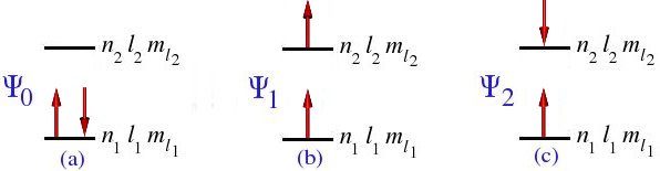
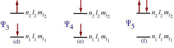
With the four spin-orbitals, we can construct six Slater determinants, or configuration functions, corresponding to the diagrammatic representations shown in Figure 4.1
(4.70)
Ψ
0
(
x
1
,
x
2
)
=
1
2
!
|
ψ
n
1
l
1
m
l
1
(
1
)
α
(
1
)
ψ
n
1
l
1
m
l
1
(
1
)
β
(
1
)
ψ
n
1
l
1
m
l
1
(
2
)
α
(
2
)
ψ
n
1
l
1
m
l
1
(
2
)
β
(
2
)
|
=
1
2
!
ψ
n
1
l
1
m
l
1
(
1
)
ψ
n
1
l
1
m
l
1
(
2
)
[
α
(
1
)
β
(
2
)
-
α
(
2
)
β
(
1
)
]
(4.71)
Ψ
1
(
x
1
,
x
2
)
=
1
2
!
|
ψ
n
1
l
1
m
l
1
(
1
)
α
(
1
)
ψ
n
2
l
2
m
l
2
(
1
)
α
(
1
)
ψ
n
1
l
1
m
l
1
(
2
)
α
(
2
)
ψ
n
2
l
2
m
l
2
(
2
)
α
(
2
)
|
=
1
2
!
[
ψ
n
1
l
1
m
l
1
(
1
)
ψ
n
2
l
2
m
l
2
(
2
)
-
ψ
n
1
l
1
m
l
1
(
2
)
ψ
n
2
l
2
m
l
2
(
1
)
]
α
(
1
)
α
(
2
)
(4.72)
Ψ
2
(
x
1
,
x
2
)
=
1
2
!
|
ψ
n
1
l
1
m
l
1
(
1
)
α
(
1
)
ψ
n
2
l
2
m
l
2
(
1
)
β
(
1
)
ψ
n
1
l
1
m
l
1
(
2
)
α
(
2
)
ψ
n
2
l
2
m
l
2
(
2
)
β
(
2
)
|
=
1
2
!
[
ψ
n
1
l
1
m
l
1
(
1
)
ψ
n
2
l
2
m
l
2
(
2
)
α
(
1
)
β
(
2
)
-
ψ
n
1
l
1
m
l
1
(
2
)
ψ
n
2
l
2
m
l
2
(
1
)
α
(
2
)
β
(
1
)
]
(4.73)
Ψ
3
(
x
1
,
x
2
)
=
1
2
!
|
ψ
n
1
l
1
m
l
1
(
1
)
β
(
1
)
ψ
n
2
l
2
m
l
2
(
1
)
α
(
1
)
ψ
n
1
l
1
m
l
1
(
2
)
β
(
2
)
ψ
n
2
l
2
m
l
2
(
2
)
α
(
2
)
|
=
1
2
!
[
ψ
n
1
l
1
m
l
1
(
1
)
ψ
n
2
l
2
m
l
2
(
2
)
α
(
2
)
β
(
1
)
-
ψ
n
1
l
1
m
l
1
(
2
)
ψ
n
2
l
2
m
l
2
(
1
)
α
(
1
)
β
(
2
)
]
(4.74)
Ψ
4
(
x
1
,
x
2
)
=
1
2
!
|
ψ
n
1
l
1
m
l
1
(
1
)
β
(
1
)
ψ
n
2
l
2
m
l
2
(
1
)
β
(
1
)
ψ
n
1
l
1
m
l
1
(
2
)
β
(
2
)
ψ
n
2
l
2
m
l
2
(
2
)
β
(
2
)
|
=
1
2
!
[
ψ
n
1
l
1
m
l
1
(
1
)
ψ
n
2
l
2
m
l
2
(
2
)
-
ψ
n
1
l
1
m
l
1
(
2
)
ψ
n
2
l
2
m
l
2
(
1
)
]
β
(
1
)
β
(
2
)
(4.75)
Ψ
5
(
x
1
,
x
2
)
=
1
2
!
|
ψ
n
2
l
2
m
l
2
(
1
)
α
(
1
)
ψ
n
2
l
2
m
l
2
(
1
)
β
(
1
)
ψ
n
2
l
2
m
l
2
(
2
)
α
(
2
)
ψ
n
2
l
2
m
l
2
(
2
)
β
(
2
)
|
=
1
2
!
ψ
n
2
l
2
m
l
2
(
1
)
ψ
n
2
l
2
m
l
2
(
2
)
[
α
(
1
)
β
(
2
)
-
α
(
2
)
β
(
1
)
]
Note that if the two sets of quantum numbers used to construct the Slater determinants are the same, i.e.,
{
n
1
,
l
1
,
m
l
1
,
m
s
1
}
=
{
n
2
,
l
2
,
m
l
2
,
m
s
2
}
,
then Ψ1 = Ψ4 = 0, Ψ0 = Ψ2 = Ψ3 = Ψ5, and our six determinants are reduced to one determinant.
[Back to Table of Contents] [Top of Chapter 4] [scienceelearning.org]
As we showed in Section 4.2, all six of the Slater determinants are eigenfunctions of
S
^
z
, but the open shell determinants (Ψ1, Ψ2, Ψ3, Ψ4) will not be eigenfunctions of
S
^
2
unless all the spins of the open shell electrons are aligned. For the closed shell determinants, Ψ1 and Ψ5, and the open shell determinants where all the spins of the open shell electrons are aligned, Ψ1 and Ψ4, we can simply apply the result of Eq. (4.55).
In other words, cases in which
S
max
=
|
M
S
|
max
.
The configuration functions, Ψ2 and Ψ3, however, are not eigenfunctions of
S
^
2
. If we apply the operator
S
^
2
to Ψ2 we find
(4.76)
S
^
2
Ψ
2
(
x
1
,
x
2
)
=
(
S
^
-
S
^
+
+
S
^
z
2
+
ℏ
S
^
z
)
Ψ
2
(
x
1
,
x
2
)
=
(
s
^
1
-
+
s
^
2
-
)
(
s
^
1
+
+
s
^
2
+
)
Ψ
2
(
x
1
,
x
2
)
=
(
s
^
1
-
+
s
^
2
-
)
ℏΨ
1
(
x
1
,
x
2
)
=
ℏ
2
[
Ψ
2
(
x
1
,
x
2
)
+
Ψ
3
(
x
1
,
x
2
)
]
where we have used the fact that
S
^
z
Ψ
2
=
0
. Similarly, if we apply
S
^
2
to Ψ3 we find
(4.77)
S
^
2
Ψ
3
(
x
1
,
x
2
)
=
(
S
^
-
S
^
+
+
S
^
z
2
+
ℏ
S
^
z
)
Ψ
3
(
x
1
,
x
2
)
=
(
s
^
1
-
+
s
^
2
-
)
(
s
^
1
+
+
s
^
2
+
)
Ψ
3
(
x
1
,
x
2
)
=
(
s
^
1
-
+
s
^
2
-
)
ℏΨ
1
(
x
1
,
x
2
)
=
ℏ
2
[
Ψ
2
(
x
1
,
x
2
)
+
Ψ
3
(
x
1
,
x
2
)
]
where, again, we have used the fact that
S
^
z
Ψ
3
=
0
.
On the other hand, if we add Eqs. (4.76) and (4.77)
(4.78)
S
^
2
[
Ψ
2
(
x
1
,
x
2
)
+
Ψ
3
(
x
1
,
x
2
)
]
=
2
ℏ
2
[
Ψ
2
(
x
1
,
x
2
)
+
Ψ
3
(
x
1
,
x
2
)
]
we see that the sum, Ψ2 + Ψ3, is an eigenstate in which S(S + 1 ) = 1 (1 + 1), and therefore S = 1.
By subtracting Eq. (4.77) from (4.76)
(4.79)
S
^
2
[
Ψ
2
(
x
1
,
x
2
)
-
Ψ
3
(
x
1
,
x
2
)
]
=
0
we see that the difference, Ψ2 - Ψ3, forms an eigenstate with S = 0. Note that the spin triplet state constructed from Ψ2 and Ψ3 is equal to
(4.80)
1
2
[
Ψ
2
(
x
1
,
x
2
)
+
Ψ
3
(
x
1
,
x
2
)
]
=
1
2
[
ψ
n
1
l
1
m
l
1
(
1
)
ψ
n
2
l
2
m
l
2
(
2
)
-
ψ
n
1
l
1
m
l
1
(
2
)
ψ
n
2
l
2
m
l
2
(
1
)
]
[
β
(
1
)
α
(
2
)
+
α
(
1
)
β
(
2
)
]
=
1
2
|
ψ
n
1
l
1
m
l
1
(
1
)
ψ
n
2
l
2
m
l
2
(
1
)
ψ
n
1
l
1
m
l
1
(
2
)
ψ
n
2
l
2
m
l
2
(
2
)
|
[
α
(
1
)
β
(
2
)
+
β
(
1
)
α
(
2
)
]
and the spin singlet is equal to
(4.81)
1
2
[
Ψ
2
(
x
1
,
x
2
)
-
Ψ
3
(
x
1
,
x
2
)
]
=
1
2
[
ψ
n
1
l
1
m
l
1
(
1
)
ψ
n
2
l
2
m
l
2
(
2
)
+
ψ
n
1
l
1
m
l
1
(
2
)
ψ
n
2
l
2
m
l
2
(
1
)
]
[
α
(
1
)
β
(
2
)
-
β
(
1
)
α
(
2
)
]
Thus, all six of the spin eigenstates constructed from the two-electron Slater determinants can be written as a product of a spatial function and a spin function. This manifestly simple decoupling of the spin degrees of freedom in the two-electron atom is not true of many-electron systems in general.
The spin-angular momentum quantum numbers of the six two-electron Slater determinants are summarized in Table 4.2
Table 4.2. The spin-angular momentum quantum numbers of two-electron wavefunctions constructed from six two-electron Slater determinants.
| | S | MS |
|---|
| | Ψ0, Ψ5,
1
2
!
[
Ψ
2
-
Ψ
3
]
| 0 | 0 |
| | Ψ1 | 1 | 1 |
| |
1
2
!
[
Ψ
2
+
Ψ
3
]
| 1 | 0 |
| | Ψ4 | 1 | -1 |
where we have included the normalization factor of
1
/
2
!
in the eigenfunctions involving two Slater determinants.
To this point, the two sets of quantum numbers n1, l1, ml1, and
n2, l2, ml2 have not been specified.
In Table 4.3, the electron configurations of six two-electron Slater determinants are shown for different values of the quantum numbers n1, l1,
n2 and l2. Note that the Slater determinants Ψ1, Ψ2, Ψ3, and Ψ4 all have the same electron configurations. The electron configuration does not specify the spin quantum numbers, or the z-component of the orbital angular momentum. Thus, there may be several different states corresponding to a given electron configuration.
Table 4.3. The electron configurations of six two-electron Slater determinants for different values of the quantum numbers n1, l1,
n2 and l2. Note that the Slater determinants Ψ1, Ψ2, Ψ3, and Ψ4 all have the same electron configurations.
|
| 1 0 | 1 0 | 1s2 | 1s2 | 1s2 | 1s2 | 1s2 | 1s2 |
| 1 0 | 2 0 | 1s2 |
1s 2s |
1s 2s |
1s 2s |
1s 2s | 2s2 |
| 1 0 | 2 1 | 1s2 | 1s 2p | 1s 2p | 1s 2p | 1s 2p | 2p2 |
| 1 0 | 3 0 | 1s2 | 1s 3s | 1s 3s | 1s 3s | 1s 3s | 3s2 |
| 1 0 | 3 1 | 1s2 | 1s 3p | 1s 3p | 1s 3p | 1s 3p | 3p2 |
| 1 0 | 3 2 | 1s2 | 1s 3d | 1s 3d | 1s 3d | 1s 3d | 3d2 |
| 1 0 | 4 0 | 1s2 | 1s 4s | 1s 4s | 1s 4s | 1s 4s | 4s2 |
| 1 0 | 4 1 | 1s2 | 1s 4p | 1s 4p | 1s 4p | 1s 4p | 4p2 |
| 1 0 | 4 2 | 1s2 | 1s 4d | 1s 4d | 1s 4d | 1s 4d | 4d2 |
| 1 0 | 4 3 | 1s2 | 1s 4f | 1s 4f | 1s 4f | 1s 4f | 4f2 |
| 2 0 | 2 0 | 2s2 | 2s2 | 2s2 | 2s2 | 2s2 | 2s2 |
[Back to Table of Contents] [Top of Chapter 4] [scienceelearning.org]
4.4.3. Orbital angular momentum.
We can use the orbital angular momentum ladder operators
(4.82)
L
^
2
=
L
^
∓
L
^
±
+
L
^
z
2
±
ℏ
L
^
z
to establish the orbital angular momentum properties of the two-electron Slater determinants in the same as was done for spin in Eqs. (4.76) - (4.79). It is useful to realize that the determinants Ψ1, Ψ2, Ψ3, and Ψ4 have the same orbital properties, and Ψ0 and Ψ5 can be obtained from Ψ2 or Ψ3 by setting
{
n
1
,
l
1
,
m
l
1
}
=
{
n
2
,
l
2
,
m
l
2
}
.
If
L
^
±
is applied to the determinantal wavefunction Ψ1 defined by Eq. (4.71) and
Figure 4.1(b) we obtain
(4.83)
L
^
±
Ψ
1
(
x
1
,
x
2
)
=
ℏ
2
[
(
l
1
∓
m
l
1
)
(
l
1
±
m
l
1
+
1
)
ψ
n
1
l
1
m
l
1
±
1
(
1
)
ψ
n
2
l
2
m
l
2
(
2
)
-
(
l
2
∓
m
l
2
)
(
l
2
±
m
l
2
+
1
)
ψ
n
1
l
1
m
l
1
(
2
)
ψ
n
2
l
2
m
l
2
±
1
(
1
)
]
α
(
1
)
α
(
2
)
+
ℏ
2
[
(
l
2
∓
m
l
2
)
(
l
2
±
m
l
2
+
1
)
ψ
n
1
l
1
m
l
1
(
1
)
ψ
n
2
l
2
m
l
2
±
1
(
2
)
-
(
l
1
∓
m
l
1
)
(
l
1
±
m
l
1
+
1
)
ψ
n
1
l
1
m
l
1
±
1
(
2
)
ψ
n
2
l
2
m
l
2
(
1
)
]
α
(
1
)
α
(
2
)
To obtain
L
^
∓
L
^
±
Ψ
1
we apply
L
^
∓
to Eq. (4.83)
(4.84)
L
^
∓
L
^
±
Ψ
1
(
x
1
,
x
2
)
=
ℏ
2
[
(
l
1
∓
m
l
1
)
(
l
1
±
m
l
1
+
1
)
+
(
l
2
∓
m
l
2
)
(
l
2
±
m
l
2
+
1
)
]
Ψ
1
(
x
1
,
x
2
)
+
ℏ
2
2
(
l
1
±
m
l
1
)
(
l
1
∓
m
l
1
+
1
)
(
l
2
∓
m
l
2
)
(
l
2
±
m
l
2
+
1
)
[
ψ
n
1
l
1
m
l
1
∓
1
(
1
)
ψ
n
2
l
2
m
l
2
±
1
(
2
)
-
ψ
n
1
l
1
m
l
1
∓
1
(
2
)
ψ
n
2
l
2
m
l
2
±
1
(
1
)
]
α
(
1
)
α
(
2
)
+
ℏ
2
2
(
l
1
∓
m
l
1
)
(
l
1
±
m
l
1
+
1
)
(
l
2
±
m
l
2
)
(
l
2
∓
m
l
2
+
1
)
[
ψ
n
1
l
1
m
l
1
±
1
(
1
)
ψ
n
2
l
2
m
l
2
∓
1
(
2
)
-
ψ
n
1
l
1
m
l
1
±
1
(
2
)
ψ
n
2
l
2
m
l
2
∓
1
(
1
)
]
α
(
1
)
α
(
2
)
If we define four new Slater determinants
(4.85)
Ψ
1∓±
(
x
1
,
x
2
)
≡
1
2
!
|
ψ
n
1
l
1
m
l
1
∓
1
(
1
)
α
(
1
)
ψ
n
2
l
2
m
l
2
±
1
(
1
)
α
(
1
)
ψ
n
1
l
1
m
l
1
∓
1
(
2
)
α
(
2
)
ψ
n
2
l
2
m
l
2
±
1
(
2
)
α
(
2
)
|
=
1
2
!
[
ψ
n
1
l
1
m
l
1
∓
1
(
1
)
ψ
n
2
l
2
m
l
2
±
1
(
2
)
-
ψ
n
1
l
1
m
l
1
∓
1
(
2
)
ψ
n
2
l
2
m
l
2
±
1
(
1
)
]
α
(
1
)
α
(
2
)
and
(4.86)
Ψ
1±∓
(
x
1
,
x
2
)
≡
1
2
!
|
ψ
n
1
l
1
m
l
1
±
1
(
1
)
α
(
1
)
ψ
n
2
l
2
m
l
2
∓
1
(
1
)
α
(
1
)
ψ
n
1
l
1
m
l
1
±
1
(
2
)
α
(
2
)
ψ
n
2
l
2
m
l
2
∓
1
(
2
)
α
(
2
)
|
=
1
2
!
[
ψ
n
1
l
1
m
l
1
±
1
(
1
)
ψ
n
2
l
2
m
l
2
∓
1
(
2
)
-
ψ
n
1
l
1
m
l
1
±
1
(
2
)
ψ
n
2
l
2
m
l
2
∓
1
(
1
)
]
α
(
1
)
α
(
2
)
then Eq. (4.84) can be written as
(4.87)
L
^
∓
L
^
±
Ψ
1
(
x
1
,
x
2
)
=
ℏ
2
[
(
l
1
∓
m
l
1
)
(
l
1
±
m
l
1
+
1
)
+
(
l
2
∓
m
l
2
)
(
l
2
±
m
l
2
+
1
)
]
Ψ
1
(
x
1
,
x
2
)
+
ℏ
2
(
l
1
±
m
l
1
)
(
l
1
∓
m
l
1
+
1
)
(
l
2
∓
m
l
2
)
(
l
2
±
m
l
2
+
1
)
Ψ
1∓±
(
x
1
,
x
2
)
+
ℏ
2
(
l
1
∓
m
l
1
)
(
l
1
±
m
l
1
+
1
)
(
l
2
±
m
l
2
)
(
l
2
∓
m
l
2
+
1
)
Ψ
1±∓
(
x
1
,
x
2
)
Using Eq. (4.82), together with Eq. (4.87) and
(4.88)
L
^
z
Ψ
1
(
x
1
,
x
2
)
=
ℏ
(
m
l
1
+
m
l
2
)
Ψ
1
(
x
1
,
x
2
)
we obtain
(4.89)
L
^
2
Ψ
1
(
x
1
,
x
2
)
=
ℏ
2
[
(
l
1
∓
m
l
1
)
(
l
1
±
m
l
1
+
1
)
+
(
l
2
∓
m
l
2
)
(
l
2
±
m
l
2
+
1
)
+
(
m
l
1
+
m
l
2
)
2
±
(
m
l
1
+
m
l
2
)
]
Ψ
1
(
x
1
,
x
2
)
+
ℏ
2
(
l
1
±
m
l
1
)
(
l
1
∓
m
l
1
+
1
)
(
l
2
∓
m
l
2
)
(
l
2
±
m
l
2
+
1
)
Ψ
1∓±
(
x
1
,
x
2
)
+
ℏ
2
(
l
1
∓
m
l
1
)
(
l
1
±
m
l
1
+
1
)
(
l
2
±
m
l
2
)
(
l
2
∓
m
l
2
+
1
)
Ψ
1±∓
(
x
1
,
x
2
)
Next, we will find cases in which the Slater determinant Ψ1, defined by Eq. (4.71) and
Figure 4.1(b), is an eigenstate of
L
^
2
.
We need only find cases in which the terms containing
Ψ
1
∓
±
and
Ψ
1
±
∓
don't contribute to Eq. (4.89). There are four obvious situations when this is true.
The first two cases were discussed before in Appendix B and restated in Eq. (4.63). For two electrons, Eq. (4.63) becomes
L
max
=
|
M
L
|
max
=
l
1
+
l
2
,
and this provides us with two situations in which Ψ1 is an eigenstate, namely,
1)
m
l
1
=
l
1
and
m
l
2
=
l
2
,
and 2)
m
l
1
=
-
l
1
and
m
l
2
=
-
l
2
.
Two more cases are: 3)
l
1
=
m
l
1
=
0
, and
4)
l
2
=
m
l
2
=
0
.
Table 4.4 was generated by plugging in the values for our four cases into Eq. (4.89).
Table 4.4. Four cases in which the two-electron Slater determinant discussed in the text is an orbital angular momentum eigenstate.
|
| l1 l1 | l2 l2 | l1 + l1 | l1 + l1 |
| l1 - l1 | l2 - l2 | l1 + l1 |
- l1 - l1 |
| 0 0 | l2
m
l
2
| l2 |
m
l
2
|
| l1
m
l
1
| 0 0 | l1 |
m
l
1
|
It was all ready mentioned in Section 4.4.2 that the example of a two-electron atom is unique in that the antisymmetric eigenstates of
L
^
2
and
S
^
2
can be written as a product of a spatial function and a spin function. If a many-electron angular momentum eigenstate in the decoupled representation is written as
Ψ
L
M
L
S
M
S
(
x
1
,
x
2
,
…
,
x
N
)
≡
〈
x
1
x
2
⋯
x
N
|
L
M
L
S
M
S
〉
, then for two-electrons it is
(4.90)
Ψ
L
M
L
S
M
S
(
x
1
,
x
2
)
=
〈
x
1
x
2
|
L
M
L
S
M
S
〉
=
〈
r
1
r
2
|L
M
L
〉
〈
σ
1
σ
2
|S
M
S
〉
=
ΨL
M
L
(
r
1
,
r
2
)
ΨS
M
S
(
σ
1
,
σ
2
)
where
(4.91)
ΨS
M
S
(
σ
1
,
σ
2
)
=
〈
σ
1
σ
2
|S
M
S
〉
=
=
{
Ψ
11
(
σ
1
,
σ
2
)
Ψ
10
(
σ
1
,
σ
2
)
Ψ
1
-
1
(
σ
1
,
σ
2
)
Ψ
00
(
σ
1
,
σ
2
)
=
{
〈
σ
1
σ
2
|
11
〉
〈
σ
1
σ
2
|
10
〉
〈
σ
1
σ
2
|
1
-
1
〉
〈
σ
1
σ
2
|
00
〉
=
{
α
(
1
)
α
(
2
)
1
2
[
α
(
1
)
β
(
2
)
+
β
(
1
)
α
(
2
)
]
β
(
1
)
β
(
2
)
1
2
[
α
(
1
)
β
(
2
)
−
β
(
1
)
α
(
2
)
]
is the spin part of the wavefunction. The minus sign − in the S = 0 function, Ψ00, is highlighted to emphasize that it is the only antisymmetric spin function of the four in Eq. (4.91). The spin triplet functions, Ψ11, Ψ10, and Ψ1-1, are all symmetric.
The spatial part of the wavefunction, for the first three cases in Table 4.4, is
(4.92)
Ψ
L
M
L
(
r
1
,
r
2
)
=
〈
r
1
r
2
|
L
M
L
〉
=
{
Ψ
l
1
+
l
2
,
l
1
+
l
2
(
r
1
,
r
2
)
Ψ
l
1
+
l
2
,
-
l
1
-
l
2
(
r
1
,
r
2
)
Ψ
l
2
m
l
2
(
r
1
,
r
2
)
=
{
〈
r
1
r
2
|
l
1
+
l
2
,
l
1
+
l
2
〉
〈
r
1
r
2
|
l
1
+
l
2
,
-
l
1
-
l
2
〉
〈
r
1
r
2
|
l
2
m
l
2
〉
=
{
1
2
[
ψ
n
1
l
1
l
1
(
1
)
ψ
n
2
l
2
l
2
(
2
)
±
ψ
n
1
l
1
l
1
(
2
)
ψ
n
2
l
2
l
2
(
1
)
]
1
2
[
ψ
n
1
l
1
-
l
1
(
1
)
ψ
n
2
l
2
-
l
2
(
2
)
±
ψ
n
1
l
1
-
l
1
(
2
)
ψ
n
2
l
2
-
l
2
(
1
)
]
1
2
[
ψ
n
1
00
(
1
)
ψ
n
2
l
2
m
l
2
(
2
)
±
ψ
n
1
00
(
2
)
ψ
n
2
l
2
m
l
2
(
1
)
]
where the plus sign in Eq. (4.92), +, corresponds to a symmetric
Ψ
L
M
L
, and the minus sign, −, corresponds to an antisymmetric
Ψ
L
M
L
. Since the overall symmetry of
Ψ
L
M
L
S
M
S
must be antisymmetric, the spin function
Ψ
00
(
σ
1
,
σ
2
)
must be combined with a symmetric
Ψ
L
M
L
[i.e., + in Eq. (4.92)].
From the triangle rule, we know that if l1 = 0, then the only possible value of L is L = l2, and all the eigenstates of
L
^
2
can be generated from Ψ1 by using the ladder operators
L
^
±
.
The expression for Ψ1 [Eq. (4.71) and Figure 4.1] becomes
(4.93)
Ψ
1
(
x
1
,
x
2
)
=
〈
x
1
x
2
|
L
=
l
2
,
M
L
=
m
l
2
,
S
=
1
,
M
S
=
1
〉
=
〈
x
1
x
2
|
l
2
m
l
2
11
〉
=
(
0
+
,
m
l
2
+
)
In the last term of Eq. (4.93), we have adopted the notation of Slater, in which the determinants are represented by their microstates [Atkins, p. 240; Lowe, p. 153; Bernath, p. 133], or the product of the diagonal elements of the Slater determinant, without the
1
/
N
!
normalization factor. In other words, the shorthand notation for the two-electron determinants is
(
m
l
1
m
s
1
,
m
l
2
m
s
2
)
,
where ms = + is used to label a spin-up electron, and
ms = − is used to label a spin-down electron [SlaterII, p. 76; Condon and Shortley, p. 169]. This is also written in the literature with a bar over the quantum number ml to label a spin-down electron, and the absence of a bar denotes the spin-up electron. Two examples that show the different notations used for the microstates are
(
0
-
,
1
+
)
=
(
0
-
,
1
)
=
s
(
1
)
p
1
(
2
)
β
(
1
)
α
(
2
)
and
(
1
+
-
1
-
)
=
(
1
,
-
1
-
)
=
p
1
(
1
)
p
-
1
(
2
)
α
(
1
)
β
(
2
)
.
To give a more specific example, let l1 = 0 and l2 = 1, corresponding to a sp configuration. When
l1 = 0 and l2 = 1,
the determinantal wavefunction Ψ1 becomes
(4.94)
Ψ
1
(
x
1
,
x
2
)
=
〈
x
1
x
2
|
L
=
1
,
M
L
=
1
,
S
=
1
,
M
S
=
1
〉
=
〈
x
1
x
2
|
11
11
〉
=
(
0
+
,
1
+
)
,
and as was all ready mentioned, all the eigenstates of
L
^
2
and
L
^
z
can be generated from Ψ1 by using the ladder operators
L
^
±
. Also, as usual, for a given eigenstate of
S
^
2
all the eigenstates of
S
^
z
can be found by using the ladder operators
S
^
±
.
For example, by using
(4.95)
S
^
±
〈
x
1
x
2
|
L
M
L
S
M
S
〉
=
ℏ
(
S
∓
M
S
)
(
S
±
M
S
+
1
)
〈
x
1
x
2
|
L
M
L
S
M
S
±
1
〉
together with the one-electron ladder operators in Eqs. (2.15) and (2.16), one can obtain
(4.96)
S
^
-
Ψ
1
(
x
1
,
x
2
)
=
S
^
-
〈
x
1
x
2
|
1111
〉
=
ℏ
2
〈
x
1
x
2
|
1110
〉
=
(
s
^
1
-
+
s
^
2
-
)
〈
r
1
r
2
|
L
=
1
,
M
L
=
1
〉
α
(
1
)
α
(
2
)
=
ℏ
〈
r
1
r
2
|
L
=
1
,
M
L
=
1
〉
[
β
(
1
)
α
(
2
)
+
α
(
1
)
β
(
2
)
]
=
ℏ
[
Ψ
2
(
x
1
,
x
2
)
+
Ψ
3
(
x
1
,
x
2
)
]
=
ℏ
[
(
0
+
,
1
-
)
+
(
0
-
,
1
+
)
]
,
and as a reminder, Ψ1, Ψ2, and Ψ3 are defined by Eqs. (4.71) - (4.73) and Figure 4.1. From Eq. (4.96), it is easy to see that
(4.97)
〈
x
1
x
2
|
1110
〉
=
1
2
[
(
0
+
,
1
-
)
+
(
0
-
,
1
+
)
]
,
and the application of the ladder operator even provides the correct normalization factor.
Similarly, for the orbital angular momentum we can use
(4.98)
L
^
±
〈
x
1
,
x
2
|
L
M
L
S
M
S
〉
=
ℏ
(
L
∓
M
L
)
(
L
±
M
L
+
1
)
〈
x
1
x
2
|
L
M
L
±
1
S
M
S
〉
together with the one-electron ladder operators in Eq. (2.91), with the substitutions
j
^
i
±
→
l
^
i
±
,
m
j
→
m
l
,
and
j
→
l
, etc., to show that
(4.99)
L
^
-
Ψ
1
(
x
1
,
x
2
)
=
L
^
-
〈
x
1
x
2
|
1111
〉
=
ℏ
2
〈
x
1
x
2
|
1011
〉
=
(
l
^
1
-
+
l
^
2
-
)
1
2
[
ψ
n
1
00
(
1
)
ψ
n
2
11
(
2
)
-
ψ
n
1
00
(
2
)
ψ
n
2
11
(
1
)
]
α
(
1
)
α
(
2
)
=
1
2
[
l
^
2
-
ψ
n
1
00
(
1
)
ψ
n
2
11
(
2
)
-
l
^
1
-
ψ
n
1
00
(
2
)
ψ
n
2
11
(
1
)
]
α
(
1
)
α
(
2
)
=
ℏ
[
ψ
n
1
00
(
1
)
ψ
n
2
10
(
2
)
-
ψ
n
1
00
(
2
)
ψ
n
2
10
(
1
)
]
α
(
1
)
α
(
2
)
=
ℏ
2
(
0
+
,
0
+
)
.
Thus,
(4.100)
〈
x
1
x
2
|
10
11
〉
=
(
0
+
,
0
+
)
.
All the spin and orbital angular momentum eigenstates of the configuration sp, shown below in Table 4.5, can be obtained by following this kind of approach. For more complicated examples, other methods, such as the use of projection operators, may be more appropriate [SlaterII, p. 79].
Table 4.5. Spin and orbital angular momentum eigenstates of the configuration sp.
|
| 1 | 1 |
∣
11
11
〉
|
(
0
+
,
1
+
)
|
| 1 | 0 |
∣
11
10
〉
|
1
2
[
(
0
+
,
1
-
)
+
(
0
-
,
1
+
)
]
|
| 1 | -1 |
∣
11
1
-
1
〉
|
(
0
-
,
1
-
)
|
| 0 | 1 |
∣
10
11
〉
|
(
0
+
,
0
+
)
|
| 0 | 0 |
∣
10
10
〉
|
1
2
[
(
0
+
,
0
-
)
+
(
0
-
,
0
+
)
]
|
| 0 | -1 |
∣
10
1
-
1
〉
|
(
0
-
,
0
-
)
|
| -1 | 1 |
∣
1
-
1
11
〉
|
(
0
+
,
-
1
+
)
|
| -1 | 0 |
∣
1
-
1
10
〉
|
1
2
[
(
0
+
,
-
1
-
)
+
(
0
-
,
-
1
+
)
]
|
| -1 | -1 |
∣
1
-
1
1
-
1
〉
|
(
0
-
,
-
1
-
)
|
| 1 | 0 |
∣
11
00
〉
|
1
2
[
(
0
+
,
1
-
)
-
(
0
-
,
1
+
)
]
|
| 0 | 0 |
∣
10
00
〉
|
1
2
[
(
0
+
,
0
-
)
-
(
0
-
,
0
+
)
]
|
| -1 | 0 |
∣
1
-
1
00
〉
|
1
2
[
(
0
+
,
-
1
-
)
-
(
0
-
,
-
1
+
)
]
|
[Back to Table of Contents] [Top of Chapter 4] [scienceelearning.org]
4.4.4. The total angular momentum J in the Russell-Saunders coupling scheme.
In the last section [Section 4.4.3], we listed in Table 4.5 all the spin and orbital angular momentum eigenstates of the configuration sp in the decoupled representation. The Clebsch-Gordan coefficients for an L = 1 orbital angular momentum vector, and a S = 1 spin angular momentum vector, shown in Table 4.6, can be used used to construct eigenstates in the coupled representation. Any set of states that are eigenstates of
L
^
2
and
S
^
2
can be referred to as a Russell-Saunders coupling scheme, or a LS-coupling scheme [Condon and Shortley, p. 189].
The set of total angular momentum eigenstates,
|
J
M
J
L
S
〉
,
shown in Table 4.6, is an example of a Russell-Saunders coupling scheme.
It can be seen from Table 4.5, that the sp configuration consists of one L = 1, S = 1, eigenspace spanned by
(2L + 1)(2S + 1) = 9 basis vectors, and a L = 1, S = 0, eigenspace spanned by (2L + 1)(2S + 1) = 3 basis vectors. Representations in these two vector spaces can be expressed symbolically, in group theory notation, as
1
⊗
1
and
1
⊗
0
,
respectively.
The triangle rule for the addition of a L = 1 vector and a S = 1 vector allows the values J = 0, 1, 2, for the total angular momentum quantum number.
The change of basis to total angular momentum eigenstates, in the Russell-Saunders coupling scheme, results in the
1
⊗
1
representation being split into three (J = 0, 1, 2), each with the degeneracy 2J + 1. The total degeneracy remains the same, however, since (2·0 + 1) + (2·1 + 1) + (2·2 + 1) = 9.
Expressed in group theory terminology,
1
⊗
1
=
2
⊕
1
⊕
0
.
The corresponding term symbols (2S + 1LJ) are 3P0, 3P1, and 3P2, respectively.
Table 4.6. The Clebsch-Gordan coefficients for L = 1, S = 1. The three possible values of J are J = 0, 1, 2, and the corresponding term symbols are 3P0, 3P1, and 3P2, respectively.
| | | |
|
L
M
L
S
M
S
〉→
|
|---|
| | |
|
J
M
J
L
S
〉
↓
|
|---|
|
∣
22
11
〉
| | 1 | 0 | 0 | 0 | 0 | 0 | 0 | 0 | 0 |
|
∣
21
11
〉
| | 0 |
1
2
|
1
2
| 0 | 0 | 0 | 0 | 0 | 0 |
|
∣
20
11
〉
| | 0 | 0 | 0 |
1
6
|
2
3
|
1
6
| 0 | 0 | 0 |
|
∣
2
-
1
11
〉
| | 0 | 0 | 0 | 0 | 0 | 0 |
1
2
|
1
2
| 0 |
|
∣
2
-
2
11
〉
| | 0 | 0 | 0 | 0 | 0 | 0 | 0 | 0 | 1 |
|
∣
11
11
〉
| | 0 |
1
2
|
-
1
2
| 0 | 0 | 0 | 0 | 0 | 0 |
|
∣
10
11
〉
| | 0 | 0 | 0 |
1
2
| 0 |
-
1
2
| 0 | 0 | 0 |
|
∣
1
-
1
11
〉
| | 0 | 0 | 0 | 0 | 0 | 0 |
1
2
|
-
1
2
| 0 |
|
∣
00
11
〉
| | 0 | 0 | 0 |
1
3
|
-
1
3
|
1
3
| 0 | 0 | 0 |
Table 4.6 can also be written in matrix form as
(4.101)
(
|
22
11
〉
|
21
11
〉
|
20
11
〉
|
2
-
1
11
〉
|
2
-
2
11
〉
|
11
11
〉
|
10
11
〉
|
1
-
1
11
〉
|
00
11
〉
)
|
J
M
J
L
S
〉
=
(
1
0
0
0
0
0
0
0
0
0
1
2
1
2
0
0
0
0
0
0
0
0
0
1
6
2
3
1
6
0
0
0
0
0
0
0
0
0
1
2
1
2
0
0
0
0
0
0
0
0
0
1
0
1
2
-
1
2
0
0
0
0
0
0
0
0
0
1
2
0
-
1
2
0
0
0
0
0
0
0
0
0
1
2
-
1
2
0
0
0
0
1
3
-
1
3
1
3
0
0
0
)
(
|
11
11
〉
|
11
10
〉
|
10
11
〉
|
11
1
-
1
〉
|
10
10
〉
|
1
-
1
11
〉
|
10
1
-
1
〉
|
1
-
1
10
〉
|
1
-
1
1
-
1
〉
)
|
L
M
L
S
M
S
〉
.
On the other hand, if S = 0, then
J
=
L
, and
the three eigenstates of the term 1P1, shown in Table 4.5, are also eigenstates of
J
^
2
.
In other words,
1
⊗
0
is irreducible. (Here we are following international convention and using the 'hat' (or circumflex),
J
^
,
to distinguish the operators
J
^
,
L
^
, and
S
^
,
from their algebraic equivalents J, L, S [36].) Thus, for the term 1P1 we simply have
(4.102)
(
|
11
10
〉
|
10
10
〉
|
1
-
1
10
〉
)
|
J
M
J
L
S
〉
=
(
|
11
00
〉
|
10
00
〉
|
1
-
1
00
〉
)
|
L
M
L
S
M
S
〉
,
and we see how the twelve basis states of the configuration sp are accounted for in the transformation between the uncoupled representation and the Russell-Saunders coupling scheme.
[Back to Table of Contents] [Top of Chapter 4] [scienceelearning.org]
4.4.5. The total angular momentum J in the jj-coupling scheme.
The change of basis between the Russell-Saunders coupling scheme and the jj-coupling scheme can be obtained by calculating the matrix elements of
L
^
2
and
S
^
2
in the jj-coupling scheme and then diagonalizing the matrices [Condon and Shortley, p. 292]. Condon and Shortley have tables of coefficients listed on page p. 294 of The Theory of Atomic Spectra. For now, we will only give an example of the transformation between the Russell-Saunders coupling scheme and the jj-coupling scheme for the sp configuration, using the results of the previous section.
Table 4.7. The transformation coefficients for the change of basis between the Russell-Saunders coupling scheme and the jj-coupling scheme for a sl configuration.
3
L
l
+
1
1
2
,
l
+
1
2
1
|
1
L
l
3
L
l
1
2
,
l
+
1
2
1
2
,
l
-
1
2
l
+
1
l
l
l
+
1
1
2
l
+
1
|
(4.103)
3
L
l
-
1
1
2
,
l
-
1
2
1
|
Table 4.8. By setting l = 1, one obtains the transformation coefficients for the change of basis between the Russell-Saunders coupling scheme and the jj-coupling scheme for a sp configuration.
3
P
2
1
2
,
3
2
1
|
1
P
1
3
P
1
1
2
,
3
2
1
2
,
1
2
2
1
1
2
1
3
|
(4.104)
3
P
0
1
2
,
1
2
1
|
If we set l = 1 in Table 4.7, then we obtain the set of coefficients in Table 4.8, and these are the ones that will be used in the following example. Furthermore, the eigenkets in the jj-coupling scheme can be written as
|
J
M
J
,
j
1
j
2
⋯
j
N
〉
for an N-electron atom, which becomes
|
J
M
J
,
j
1
j
2
〉
for our example of a two-electron atom. When the eigenstates of the terms 3P2, 1P1, 3P1, and
3P0,
in Table 4.8, are written out explicity, we have
(4.105)
(
|
22
1
2
3
2
〉
|
21
1
2
3
2
〉
|
20
1
2
3
2
〉
|
2
-
1
1
2
3
2
〉
|
2
-
2
1
2
3
2
〉
)
|
J
M
J
j
1
j
2
〉
=
(
|
22
11
〉
|
21
11
〉
|
20
11
〉
|
2
-
1
11
〉
|
2
-
2
11
〉
)
|
J
M
J
L
S
〉
,
|
00
1
2
1
2
〉
|
J
M
J
j
1
j
2
〉
=
|
00
11
〉
|
J
M
J
L
S
〉
,
and
(4.106)
(
|
11
1
2
3
2
〉
|
10
1
2
3
2
〉
|
1
-
1
1
2
3
2
〉
|
11
1
2
1
2
〉
|
10
1
2
1
2
〉
|
1
-
1
1
2
1
2
〉
)
|
J
M
J
j
1
j
2
〉
=
(
2
3
0
0
1
3
0
0
0
2
3
0
0
1
3
0
0
0
2
3
0
0
1
3
1
3
0
0
2
3
0
0
0
1
3
0
0
2
3
0
0
0
1
3
0
0
2
3
)
(
|
11
10
〉
|
10
10
〉
|
1
-
1
10
〉
|
11
1
1
〉
|
10
11
〉
|
1
-
1
11
〉
)
|
J
M
J
L
S
〉
.
It is easy to see from Eq (4.106) how, in general, states with different values of L and different values of S are coupled together to form eigenkets in the jj-coupling scheme.
![[Note]](images/note.png) | |
|---|
| ...to be continued. |
[Back to Table of Contents] [Top of Chapter 4] [scienceelearning.org]
[
Back to Table of Contents] [Top of
Chapter 4] [
scienceelearning.org]